Alejandro Garcés Ruiz - Mathematical Programming for Power Systems Operation

where f represents operative costs, h are costs of turning-ON and turning-OFF, r are starting ramps, and p min, p maxare the operation limits of each unit. Binary problems are usually difficult; however, it is possible to find either convex approximation or MILP equivalents as presented in Chapter 5.

We can use the same convex approximations of the optimal power flow problem in problems such as the optimal placement of distributed generation in power distribution networks. The problem consists of determining the placement and capacity of distributed generation, subject to physical constraints, such as voltage regulation and transmission lines’ capacity. Besides, the problem includes binary constraints related to the placement of the distributed generation. The objective function is usually total power loss, although other objectives, such as reliability and optimal costs, are also suitable.

Another binary problem closely related to the OPF is the optimal placement of capacitors. In this problem, fixed or variable capacitors are placed along the primary feeder to minimize power loss. The capacitors’ location and the number of fixed capacitors in each node are binary variables considered in the model. Chapter 11examines the optimal placement of capacitors and the optimal placement of distributed generation.

The topology of a grid is not constant, especially in power distribution networks. There are several sectionalizing switches along with the primary feeders that permit transferring load among circuits. A feeder reconfiguration is an operating model that determines the optimal topology to minimize power loss. This model is non-linear, non-convex, and binary. In addition, it has a constraint related to the connectivity and radiality of the graph that is tricky to represent in equations. All these aspects are studied in Chapter 11.

Like the state estimation is the inverse of the optimal power problem, there is a problem that can be considered as the inverse of the primary feeder reconfiguration. It is the topology identification in power distribution grids, which takes measurements of current and voltages in different parts of the grid and determines the state of each sectionalizing switch. This problem is studied in Chapter 12.

Phase balancing is a combinatorial problem that consists of phase swapping of the loads and generators to reduce power loss. Despite being a classic problem, it is still relevant since the unbalance is a common phenomenon in microgrids, especially when single-phase photovoltaic units are included. Because it is a combinatorial problem, phase balancing requires heuristic algorithms with high computational effort. However, it is possible to generate simplified instances of the problem, as presented in Chapter 13.

Each three-phase node has six possible configurations as depicted in Figure 1.6. The problem consists of defining the phase in which each load or generator is connected in order to reduce the grid’s total losses. Therefore, the problem is combinatorial since there are 6 npossible configurations, where n is the number of three-phase nodes. The problem is nontrivial even in small networks; for example, a microgrid with 10 nodes will have 6 × 10 7possible configurations.

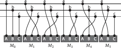
Figure 1.6 Set of possible configurations in a three-phase node.

Phase-balancing problems appear in many applications such as aircraft electric systems [4], and in power distribution grids with high penetration of electric vehicles [5]. Due to its combinatorial nature, the problem necessitates the use of heuristics [6], and meta-heuristics [7] as well as expert systems [8]. Modern approaches include the uncertainty associated to the load and generator [9].

A receding horizon control can implement most of the optimization algorithms presented in this book. Figure 1.7 depicts the main architecture for this simple but powerful strategy, for real-time implementation of operation models. These optimization models may be the optimal power flow, economic dispatch, energy storage management, or a mixed model that includes multiple models. An unbiased forecast predicts variables such as wind speed, solar radiation, and power demand. Moreover, a state estimator gives accurate measurements of the system variables.

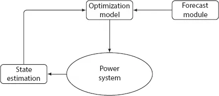
Figure 1.7 A possible architecture for implementing an optimization model for power systems operation.

( Equation 1.10) represents the optimization model, where x is the vector of decision variables for each time t , and α are the parameters predicted by the forecast module. Of course, this forecast may change since renewable resources and loads may be highly variable in modern power systems. Therefore, the optimization model must be continuously executed and the solution updated.

(1.10)

In many cases, the forecast has an error that introduces uncertainty in the model. Either stochastic or robust optimization is a suitable option to face this uncertainty. Chapter 6presents the latter option.

Python is a general programming language that is gaining attention in power systems optimization. Although it is neither a mathematical software nor an algebraic modeling language, it has many free tools for solving optimization problems. Moreover, there are many other tools for data manipulation, plotting, and integration with other software. Hence, it is a convenient platform for solving practical problems and integrate different resources 3.

We use a module named CvxPy (cvxpy) [10] that allows to solve convex and mixed-integer convex optimization problems; this module, together with NumPy, MatplotLib, and Pandas, forms a robust platform for solving all types of optimization problems in power systems applications. Let us consider, for instance, the following optimization problem:

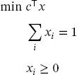(1.11)

where x ∈ 6and c = (5, 3, 2, 4, 8, 7) ⊤. A model in CvxPy for this problem looks as follows:

importnumpy asnp importcvxpy ascvx c = np.array([5,3,2,4,8,7]) x = cvx.Variable(6) objective = cvx.Minimize(c.T * x) constraints = [ sum(x) == 1, x >= 0] Model = cvx. Problem(objective,constraints) Model. solve()

Without much effort, we can identify variables, the objective function, and constraints. This neat code feature is an essential aspect of Python and CvxPy. After the problem is solved, we can make additional analyses using the same platform. This combination of tools is, of course, a great advantage; however, we must avoid any fanaticism for software. There are many programming languages and many modules for mathematical optimization. What is learned in this book may be translated to any other language. The problem is the same, although its implementation may change from one platform to another.