Alejandro Garcés Ruiz - Mathematical Programming for Power Systems Operation

We made a great effort in making the examples as simple as possible (we call them toy-models ). This approach allows us to understand each problem individually and do numerical experiments. Real operation models may include different aspects of these toy-models; for instance, they may combine economic dispatch, optimal power flow, and state estimation. These models are highly involved with thousands of variables and constraints. Nevertheless, they can be solved using the same paradigm presented in this book.

1 1We incorporate uncertainty in the models using robust optimization. Chapter 6is dedicated to this aspect.

2 2It is usual to consider the Frobenius norm as explained in Chapter 12.

3 3See appendix C for a brief introduction to Python.

Learning outcomes

By the end of this chapter, the student will be able to:

Establish first-order conditions for locally optimal solutions.

Solve unconstrained optimization problems, using the gradient method, implemented in Python.

Solve equality-constrained optimization problems, using Newton’s method implemented in Python.

Sets and functions are familiar concepts in mathematics. A set is a well-defined collection of distinct objects, considered an object in its own right. A function is a map that takes objects from one set (i.e., input or domain) and returns an object in another set (i.e., output or image). An optimization problem consists of finding the best object in the output set and its corresponding input, as shown schematically in Figure 2.1. The input set Ω is called the set of feasible solutions, and the best object corresponds to a minimum or a maximum, according to an objective function f:Ω⊆Rn→R.

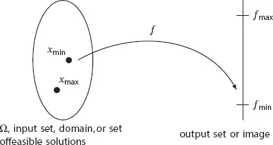
Figure 2.1 Representation of the sets related to a general optimization problem.

Solving an optimization problem implies not only to find the value of the objective function (e.g., f minor f max) but also the value x , at the input set Ω (e.g., x min, x max). These values are represented as follows:

(2.1)

(2.2)

Notice that f minand f maxare numbers whereas x minand x maxare vectors. The following example shows the difference between min and argmin (the same applies for max and argmax ).

Let us consider four simple optimization problems and their respective solution, namely 1:

(2.3)

(2.4)

(2.5)

(2.6)

As aforementioned, the operator min returns a number while the operator argmin can return a vector. Two or more points could produce the same minimum. In that case, the argmin is not unique.

But, what exactly does it mean the best solution? And, what characteristics should have both the sets and the functions involved in the problem? Some mathematical sophistication is required to answer these questions. Finding the best solution in a set implies comparing one element with the rest of the set elements. A comparison is a relation of the form x ≤ y or x ≥ y . However, not all sets allow these types of comparisons; those that enable it are called ordered sets. For instance, the real numbers and the integer numbers are all ordered set. However, complex numbers are non-ordered because such a comparison is not possible (what number is higher: zA = 1 + j or iB = 1 − j ?).

The objective function establishes a criterion of comparison. Therefore, its output must be an ordered set. Nevertheless, the input set may be ordered or non-ordered; it depends on the problem’s representation. For example, the optimal power flow in power distribution networks targets an ordered set since the active power losses belongs to the real numbers; however, the input may be represented as a vector (v,θ)∈R2×n or as a set of phasors vejθ∈Cn). The former is an ordered set, whereas the latter is non-ordered. Other possible representations can be the set of positive definite matrices or positive polynomials, as presented in Chapter 10. In conclusion, the objective function must point to an ordered set, but the input set (i.e., the set of feasible solutions) can be any arbitrary set.

We usually compare values in the output set since our objective is to minimize or maximize the objective function. It is also possible to compare values in Ω when it is an ordered set. However, a comparison between elements of the input set may be different in the output set. A function f is monotone (or monotonic) increasing, if x ≤ y implies that f ( x ) ≤ f ( y ), that is to say, the function preserves the inequality. Similarly, a function is monotone decreasing if x ≤ y implies that f ( x ) ≥ f ( y ), that is to say, the function reverses the identity.

The function f ( x ) = x 2is not monotone; for example −3 ≤ 1 but f(−3)≰f(1). Nevertheless, the function is monotone increasing in R+ +. In this set, 4 ≤ 8 implies that f ( x ) ≤ f ( y ) since both 4 and 8 belong to R+ +.

An ordered set Ω ∈ nadmits the following definitions:

Supreme: the supreme of a set, denoted by sup(Ω), is the minimum value greater than all the elements of Ω.

Infimum: the infimum of a set, denoted by inf(Ω), is the maximum value lower than all the elements of Ω.

The supreme and the infimum are closely related to the maximum and the minimum of a set. They are equal in most practical applications. The main difference is that the infimum and the supreme can be outside the set. For example, the supreme of the set Ω = { x : 3 ≤ x ≤ 5} is 5 whereas its maximum does not exists. It may seem like a simple difference, but several theoretical analyzes require this differentiation.