Alejandro Garcés Ruiz - Mathematical Programming for Power Systems Operation

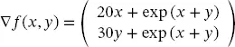
Consider the following optimization problem:

(2.31)

The gradient of this function is presented below:

(2.32)

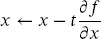
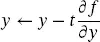
We require to find a value ( x , y ) such that this gradient is zero. Therefore, we use the gradient method. The algorithm starts from an initial point (for example x = 10, y = 10) and calculate new points as follows:

(2.33)

(2.34)

This step can be implemented in a script in Python, as presented below:

importnumpy asnp x = 10 y = 10 t = 0.03 fork in range(50): dx = 20*x + np.exp(x+y) dy = 30*y + np.exp(x+y) x += -t*dx y += -t*dy print('grad:',np. abs([dx,dy])) print('argmin:',x,y)

In the first line, we import the module NumPy with the alias np. This module contains mathematical functions such as sin, cos, exp, ln among others. The gradient introduces two components dx and dy, which are evaluated in each iteration and added to the previous point (x,y). We repeat the process 50 times and print the value of the gradient each iteration. Notice that all the indented statements belong to the for-statement, and hence the gradient is printed in each iteration. In contrast, the argmin is printed only at the end of the process.

Python allows calculating the gradient automatically using the module AutoGrad. It is quite intuitive to use. Consider the following script, which solves the same problem presented in the previous example:

importautograd.numpy asnp fromautograd importgrad # gradient calculation deff(x): z = 10.0*x[0]**2 + 15*x[1]**2 + np.exp(x[0]+x[1]) returnz g = grad(f) # create a funtion g that returns the gradient x = np.array([10.0,10.0]) t = 0.03 fork in range(50): dx = g(x) x = x -t*dx print('argmin:',x)

In this case, we defined a function f and its gradient g where ( x , y ) was replaced by a vector ( x 0, x 1). The module NumPy was loaded using autograd.numpy to obtain a gradient function automatically. The code executes the same 50 iterations, obtaining the same result. The reader should execute and compare the two codes in terms of time calculation and results.

Consider a small photovoltaic system formed by three solar panels A , B , and C , placed as depicted in Figure 2.6. Each solar system has a power electronic converter that requires to be connected to a common point E before transmitted to the final user in D . The converters and the user’s location are fixed, but the common point E can be moved at will. The coordinates of the solar panels and the final user are A = (0, 40), B = (20, 70), C = (30, 0), and D = (100, 50) respectively.

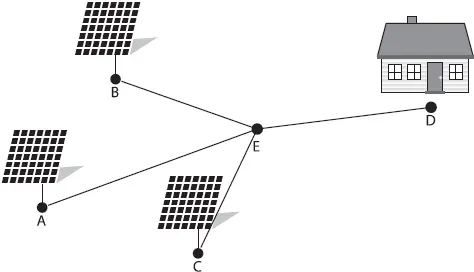
Figure 2.6 A small photovoltaic system with three solar panels.

The cost of the cables is different since each cable carries different current. Our objective is to find the best position of E in order to minimize the total cost of the cable. Therefore, the following unconstrained optimization problem is formulated:

(2.35)

where costij¯ is the unitary cost of the cable that connects the point i and j , and ij¯ is the corresponding length.

The costs of the cables are costAE¯ = 12, costBE¯ = 13, costCE¯=11 and costDE¯=18 The distance between any two points U = ( u 0, u 1) and V = ( v 0, v 1) is given by the following expression:

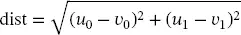(2.36)

This equation is required several times; thus, it is useful to define a function, as presented below:

importnumpy asnp A = (0,40) B = (20,70) C = (30,0) D = (100,50) defdist(U,V): returnnp.sqrt((U[0]-V[0])**2 + (U[1]-V[1])**2) P = [31,45] f = 12*dist(P,A) + 13*dist(P,B) + 11*dist(P,C) + 18*dist(P,D) print(f)

The function is evaluated in a point P = (10, 10) to see its usage 2. The value of the objective function is easily calculated as function of dist( U , V ). Likewise, the gradient of f is defined as function of the gradient of dist( U , V ) with V fixed, as presented below:

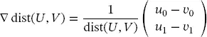(2.37)

then,

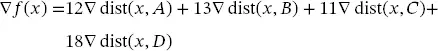(2.38)

These functions are easily defined in Python as follows:

defg_d(U,V): "gradient of the distance" return[U[0]-V[0],U[1]-V[1]]/dist(U,V) defgrad_f(E): "gradient of the objective function" return12*g_d(E,A)+13*g_d(E,B)+11*g_d(E,C)+18*g_d(E,D)

Now the gradient method consists in applying the iteration given by ( Equation 2.30), as presented below:

t = 0.5

E = np.array([10,10])

for iter in range(50): E = E -t*grad_f(E) f = 12*dist(E,A) + 13*dist(E,B) + 11*dist(E,C) + 18*dist(E,D) print("Position:",E) print("Gradient",grad_f(E)) print("Cost",f)

In this case, t = 0.5 and a initial point E = (10, 10) with 50 iterations were enough to find the solution. The reader is invited to try with other values and analyze the effect on the algorithm’s convergence.

The step t is very important for the convergence of the gradient method. It can be constant or variable, according to a well-defined update rule. There are many variants of this algorithm, most of them with sophisticated ways to calculate this step 3. A plot of ‖∇ f ‖ versus the number of iterations may be useful for determining the optimal value of t and showing the convergence rate of the algorithm, as presented in the next example. We expect a linear convergence for the gradient method, although the algorithm can lead to oscillations and even divergence if the parameter t is not selected carefully. Fortunately, there are modules in Python that make this work automatically.