Alejandro Garcés Ruiz - Mathematical Programming for Power Systems Operation
Здесь есть возможность читать онлайн «Alejandro Garcés Ruiz - Mathematical Programming for Power Systems Operation» — ознакомительный отрывок электронной книги совершенно бесплатно, а после прочтения отрывка купить полную версию. В некоторых случаях можно слушать аудио, скачать через торрент в формате fb2 и присутствует краткое содержание. Жанр: unrecognised, на английском языке. Описание произведения, (предисловие) а так же отзывы посетителей доступны на портале библиотеки ЛибКат.
- Название:Mathematical Programming for Power Systems Operation
- Автор:
- Жанр:
- Год:неизвестен
- ISBN:нет данных
- Рейтинг книги:4 / 5. Голосов: 1
-
Избранное:Добавить в избранное
- Отзывы:
-
Ваша оценка:
Mathematical Programming for Power Systems Operation: краткое содержание, описание и аннотация
Предлагаем к чтению аннотацию, описание, краткое содержание или предисловие (зависит от того, что написал сам автор книги «Mathematical Programming for Power Systems Operation»). Если вы не нашли необходимую информацию о книге — напишите в комментариях, мы постараемся отыскать её.
, Professor Alejandro Garces delivers a comprehensive overview of power system operations models with a focus on convex optimization models and their implementation in Python. Divided into two parts, the book begins with a theoretical analysis of convex optimization models before moving on to related applications in power systems operations.
The author eschews concepts of topology and functional analysis found in more mathematically oriented books in favor of a more natural approach. Using this perspective, he presents recent applications of convex optimization in power system operations problems.
Mathematical Programming for Power System Operation with Applications in Python A thorough introduction to power system operation, including economic and environmental dispatch, optimal power flow, and hosting capacity Comprehensive explorations of the mathematical background of power system operation, including quadratic forms and norms and the basic theory of optimization Practical discussions of convex functions and convex sets, including affine and linear spaces, politopes, balls, and ellipsoids In-depth examinations of convex optimization, including global optimums, and first and second order conditions Perfect for undergraduate students with some knowledge in power systems analysis, generation, or distribution,
is also an ideal resource for graduate students and engineers practicing in the area of power system optimization.
Mathematical Programming for Power Systems Operation — читать онлайн ознакомительный отрывок
Ниже представлен текст книги, разбитый по страницам. Система сохранения места последней прочитанной страницы, позволяет с удобством читать онлайн бесплатно книгу «Mathematical Programming for Power Systems Operation», без необходимости каждый раз заново искать на чём Вы остановились. Поставьте закладку, и сможете в любой момент перейти на страницу, на которой закончили чтение.
Интервал:
Закладка:
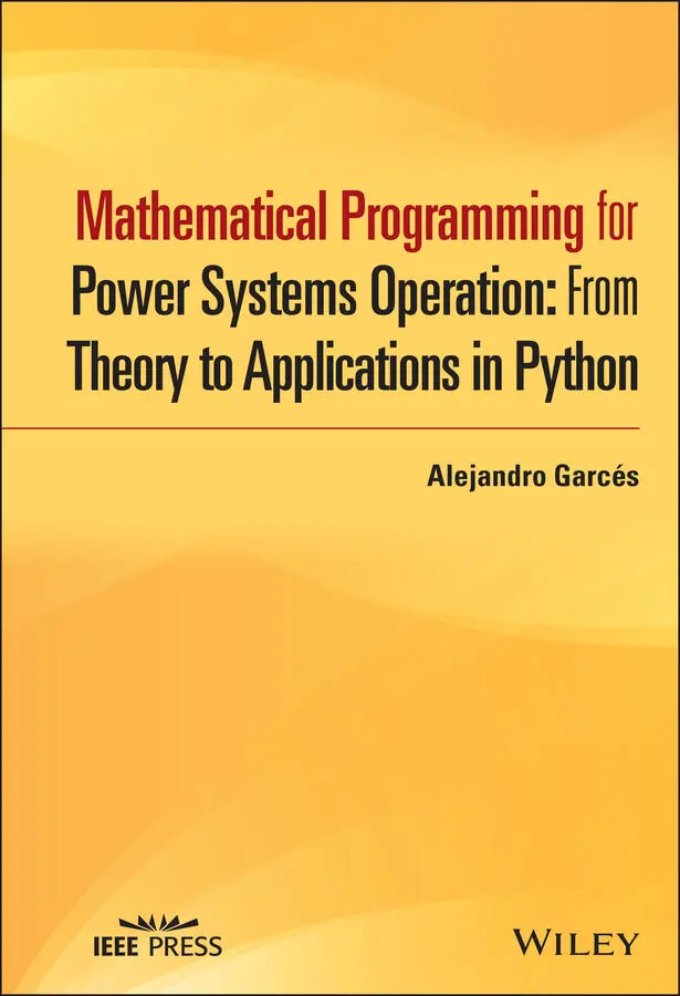
 (2.53)
 (2.54)
This iteration is the primary Newton’s method. Compared to the gradient method, this method is faster since it includes information from the second derivative 5. In addition, Newton’s method does not require defining a step t as in the gradient method. However, each iteration of Newton’s method is computationally expensive since it implies the formulation of a jacobian and solves a linear system in each iteration.
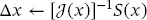
Example 2.9
Consider the following optimization problem:
 (2.55)
Its corresponding lagrangian is presented below:
 (2.56)
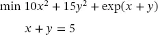
and the optimal conditions forms the following set of algebraic equations:
 (2.57)
The corresponding Jacobian is the following matrix:
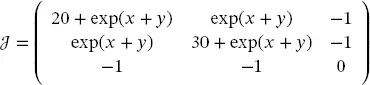 (2.58)
It is possible to formulate Newton’s method using the information described above. The algorithm implemented in Python is presented below:
importnumpy asnp defFobj(x,y): "Objective funcion" return10*x**2 + 15*y**2 + np.exp(x+y) defGrad(x,y,z): "Gradient of Lagrangian" dx = 20*x + np.exp(x+y) + z dy = 30*y + np.exp(x+y) + z dz = x + y - 5 returnnp.array([dx,dy,dz]) defJac(x,y,z): "Jacobian of Grad" p = np.exp(x+y) returnnp.array([[20+p,p,1],[p,30+p,1],[1,1,0]]) (x,y,z) = (10,10,1) # initial condition G = Grad(x,y,z) whilenp.linalg.norm(G) >= 1E-8: J = Jac(x,y,z) step = -np.linalg.solve(J,G) (x,y,z) = (x,y,z) + step G = Grad(x,y,z) print('Gradient: ',np.linalg.norm(G)) print('Optimum point: ', np.round([x,y,z],2)) print('Objective function: ', Fobj(x,y))
In this case, we used a tolerance of 10 −3. The algorithm achieves convergence in few iterations, as the reader can check by running the code.

2.8 Further readings
This chapter presented basic optimization methods for constrained and unconstrained problems. Conditions for convergence of these algorithms were not presented here. However, they are incorporated into modules and solvers called for a modeling/programming language such as Python. Our approach is to use these solvers and concentrate on studying the characteristics of the models. Readers interested in details of the algorithms are invited to review [12] and [11], for a formal analysis of convergence; other variants of the algorithms can be found in [13]. Moreover, a complete review of Lagrange multipliers can be studied in [14].
This chapter is also an excuse for presenting Python’s features as programming and modeling language. The reader can review Appendix C for more details about each of the commands used in this section.
2.9 Exercises
1 Find the highest and lowest point, of the set given by the intersection of the cylinder x2 + y2 ≤ 1 with the plane x + y + z = 1, as shown in Figure 2.8. Figure 2.8 Intersection of an affine space with a cylinder.
2 What is the new value of zmax and zmin, if the cylinder increases its radius in a small value, that is, if the radius changes from (r = 1) to (r = 1 + Δr) (Consider the interpretation of the Lagrange multipliers).
3 The following algebraic equation gives the mechanical power in a wind turbine: (2.59)where P is the power extracted from the wind; ρ is the air density; Cp is the performance coefficient or power coefficient; λ is the tip speed ratio; v is the wind velocity, and A is the area covered by the rotor (see [15] for details). Determine the value of λ that produce maximum efficiency if the performance coefficient is given by (Equation 2.60): (2.60)Use the gradient method, starting from λ = 10 and a step of t = 0.1. Hint: use the module SymPy to obtain the expression of the gradient.
4 Solve the following optimization problem using the gradient method: (2.61)Depart from the point (0, 0) and use a fixed step t = 0.8. Repeat the problem with a fixed step t = 1.1. Show a plot of convergence.
5 Solve the following optimization problem using the gradient method. (2.62)where 1n is a column vector of size n, with all entries equal to 1; b is a column vector such that bk = kn2; and H is a symmetric matrix of size n × n constructed in the following way: hkm = (m + k) / 2 if k ≠ m and hkm = n2 + n if k = m. Show the convergence of the method for different steps t and starting from an initial point x = 0. Use n = 10, n = 100, and n = 1000. All index k or m starts in zero.
6 Show that Euclidean, Manhattan, and uniform norms fulfill the four conditions to be considered a norm.
7 Consider a modified version of Example 2.6, where the position of the common point E must be such that xE = yE. Solve this optimization problem using Newton’s method.
8 Solve the problem of Item 4 with the following constraint (use Newton’s method): (2.63)
9 Solve problem of Item 5 including the following constraint (use Newton’s method): (2.64)
10 Newton’s method can be used to solve unconstrained optimization problems. Solve the following problem using Newton’s method and compare the convergence rate and the solution with the gradient method. (2.65)
Notes
1 1At this point, the only tool we have to check these results is plotting the function and locating the optimum.
2 2Notice P is defined in a line outside the function definition. Recall that x2 is represented as x**2 in Python (see Appendix C)
3 3A complete discussion about the calculation of t is beyond this book’s objectives. Interested readers can consult the work of Nesterov and Nemirovskii, in [11] and [12].
4 4Again, a classic method that became more important with the advent of the computer.
5 5The jacobian matrix of S is equivalent to the hessian matrix of f.
Конец ознакомительного фрагмента.
Текст предоставлен ООО «ЛитРес».
Прочитайте эту книгу целиком, купив полную легальную версию на ЛитРес.
Безопасно оплатить книгу можно банковской картой Visa, MasterCard, Maestro, со счета мобильного телефона, с платежного терминала, в салоне МТС или Связной, через PayPal, WebMoney, Яндекс.Деньги, QIWI Кошелек, бонусными картами или другим удобным Вам способом.
Интервал:
Закладка:
Похожие книги на «Mathematical Programming for Power Systems Operation»
Представляем Вашему вниманию похожие книги на «Mathematical Programming for Power Systems Operation» списком для выбора. Мы отобрали схожую по названию и смыслу литературу в надежде предоставить читателям больше вариантов отыскать новые, интересные, ещё непрочитанные произведения.


Обсуждение, отзывы о книге «Mathematical Programming for Power Systems Operation» и просто собственные мнения читателей. Оставьте ваши комментарии, напишите, что Вы думаете о произведении, его смысле или главных героях. Укажите что конкретно понравилось, а что нет, и почему Вы так считаете.