Alejandro Garcés Ruiz - Mathematical Programming for Power Systems Operation

All applications are presented in Python, which is a language that is becoming more important in power systems applications. Students are not expected to have previous knowledge in Python, although basic concepts about programming (in any language) are helpful. Our methodology is based on many examples and toy-models . We made a great effort in showing the most simple model with a clean code. Of course, these toy-models are an oversimplification of the real problem; however, they allow us to understand the model and its coding. In practice, we may have complex models that combine different aspects such as the economic dispatch, the unit commitment and/or the optimal power flow. A real operation model may require a sophisticated platform that integrates the model with the supervisory control and data acquisition system (SCADA) operating in real-time. The development of such a real industrial model is beyond the objectives of this book.

Learning outcomes

By the end of this chapter, the student will be able to:

Identify problems related to power systems operation.

Link mathematical optimization models to power systems operation problems.

Mathematical optimization is a fundamental tool for the electrical supply chain, from generation through transmission, distribution, and end-use. It may also be used, in different time frames, from a few milliseconds to several years. This book concentrates on optimization problems for power systems operation. These problems are usually continuous and have a time frame from several minutes to one day. Optimization problems with faster dynamics lie in the control and stability analysis, whereas problems with slower dynamics are planning problems.

Mathematical optimization problems associated with power system operation have existed since the beginning of operations research as an independent area, back in the middle of the 20th century. However, modern technologies such as renewable energies and electric vehicles; and current concepts, such as smart-grids, active distribution networks, and microgrids, have created a renewed interest in mathematical optimization applied to power systems. Smart-grids implicate a massive use of technologies such as power electronics, communications, and advanced metering. However, the smart aspect of these grids comes from mathematical techniques such as mathematical optimization, that manage these technologies, in order to improve the efficiency, reliability, security, and resilience of the system.

Figure 1.1 depicts schematically four common types of mathematical optimization models. These are linear programming (LP), mixed-integer linear programming (MIP), non-linear programming (NLP), and mixed-integer non-linear programming (MINLP). Another classification is to separate them into convex and non-convex problems. The former include LPs and some NLPs; the latter is the rest of the problems. Convex problems are well-behaved in the sense that they have theoretical guarantees, such as global optimum and practical algorithms with fast convergence rate. The first part of the book presents these theoretical aspects. However, not all power systems operation problems are convex; therefore, we need to develop convex approximations for those problems, most of them based on conic optimization as presented in Chapter 5.

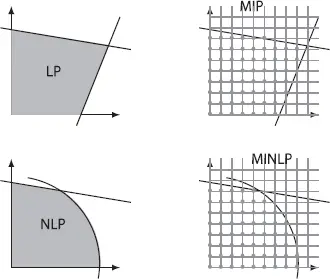
Figure 1.1 Types of optimization models.

A power system is quite complex, and therefore, modeling and implementing mathematical optimization problems are equally complex. We need to gain experience in the complex art of modeling and solving mathematical optimization problems for power system applications. Our approach is to create toy-models for each problem. These are simplified models that allow us to understand the central issues and do numerical experiments. In the following sections, we briefly describe each of these toy-models, explained in detail in the second part of the book.

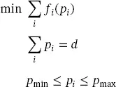
The economic and environmental dispatch of thermal units is one of the most classic problems in power systems operation. It consists of minimizing the operating costs or the total CO 2emissions, subject to physical constraints such as the power balance and the maximum generation capacity. For the economic dispatch, each generation unit has a cost function fi , which is usually quadratic and depends on the power generated by each unit. Thus, the objective is to minimize the total cost (or emissions), subject to power balance, as presented below:

(1.1)

where pi is the power generated by each thermal unit, and d is the total demand. Environmental dispatch introduces quadratic or exponential functions in the objective function, but the problem’s structure is the same. Moreover, power flow constraints can be introduced into the model, although, in that case, it is more precise to name the problem as an optimal power flow (OPF). Chapter 7presents the economic and environmental dispatches, while Chapter 10presents the OPF problem.

Another problem closely related to the economic dispatch of thermal units is the unit commitment. This problem considers not only the operating costs but also the start-up and shut-down costs of thermal units. Therefore, the problem becomes binary and dynamic. This problem is studied in Chapter 8.

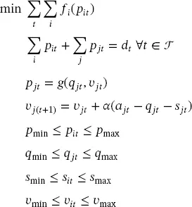
The economic dispatch problem may include hydroelectric power plants; said plants, generate two fundamental changes into the model. On the one hand, the model becomes dynamic since current operational decisions affect the future operation of the system. On the other hand, the problem becomes stochastic, because the inflows are usually random variables, especially in long-term models. The later aspect is usually solved by an accurate forecasting of the loads and the inflows; hence, it is possible to formulate a deterministic problem, called hydrothermal dispatch or hydrothermal coordination. The basic model has the following structure, namely:

(1.2)

Where i represents thermal units and j enumerates hydroelectric units; t represents the time, thus, pit is the power generated by the thermal unit i at time t . The values of ajt , vjt , pjt , qjt and sjt are respectively, the inflow, volume, power, outflow, and spillage of the hydroelectric unit j at time t . Figure 1.2, which is self-explanatory, shows these variables.

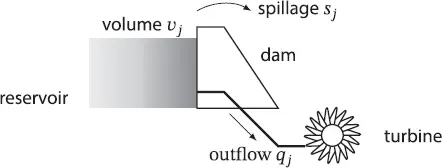
Figure 1.2 Schematic representation of the variables associated to a hydroelectric generation unit.

In this model, g represents the relation between generated power, outflow, and water volume stored in the dam. Although the planning horizon may be of short-term (1 day to 1 week), medium-term (1 month), or long-term (1 or more years), we are interested only in the short-term model. As aforementioned, the problem may be stochastic since power demands dt and inflows ajt are all random variables. However, a determinist model is suitable to understand the problem and its practical implementation. The situation becomes even more problematic when introducing other renewable energies, such as wind generation and photovoltaic solar generation. Chapter 9presents the hydrothermal dispatch problem.