Joel P. Dunsmore - Handbook of Microwave Component Measurements

(1.47)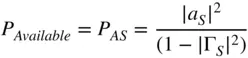

where Γ Sis computed as in Eq. (1.24)as

(1.48)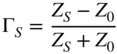

This maximum power is delivered to the load when the load impedance is the conjugate of the source impedance, .

The power that is absorbed by an arbitrary load is called the delivered power , and it is computed directly from the difference between the incident and reflected power.

(1.49)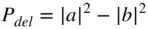

For most cases, this is the power parameter that is of greatest interest. In the case of a transmitter, it represents the power that is delivered to the antenna, for example, which in turn is the power radiated less the resistive loss of the antenna.

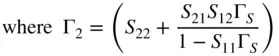
A special case of available power is the power available from the output of a network, when the network is connected an arbitrary source. In this case, the available power is only a function of the network and the source impedance and is not a function of the load impedance. It represents the maximum power that could be delivered to a load under the condition that the load impedance was ideally matched and can be found by noting that the available output power is similar to Eq. (1.47)but with the source reflection coefficient replaced by the output reflection coefficient of the network Γ 2from Eq. (1.30)such that

(1.50)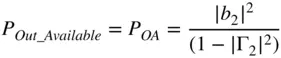

When a 2‐port network is connected to a generator with arbitrary impedance, the output scattered wave into matched load is

(1.51)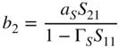

Here the incident wave is represented as a Srather than a 1as an indication that the source is not matched, and Γ 1is defined by Eq. (1.27). The output power incident to the load is

(1.52)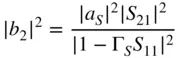

Combining Eqs. (1.52)and (1.50), the available power at the output from a network that is driven from a generator with source impedance of Γ Sis

(1.53)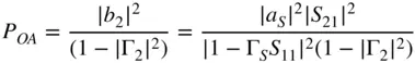

With Γ 2defined as in Eq. (1.30).

Available gain is the gain that an amplifier can provide to a conjugately matched load from a source or generator of a given impedance and is computed with the formula

(1.54)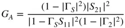

Other derived values such as maximum available gain and maximum stable gain are discussed in detail in Chapter 6.

For a receiver, the key figure of merit is its sensitivity, or the ability to detect small signals. This is limited by the intrinsic noise of the device itself, and for amplifiers and mixers, this is represented as noise figure. Noise figure is defined as a signal‐to‐noise ratio at the input divided by signal to noise at the output expressed in dB.

(1.55)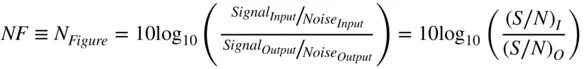

Its related value, noise factor, which is unitless, is

(1.56)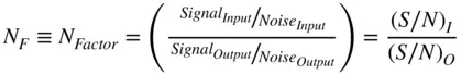

Here the signal and noise values are represented as a power; traditionally, this is available power, but incident power can be used as well with a little care. Rearranging Eq. (1.55), one can obtain

(1.57)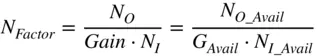

In most cases, the input noise is known very well, as it consists only of thermal noise associated with the temperature of the source resistance. This is the noise available from the source and can be found from

(1.58)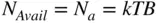

where k is Boltzmann's constant (1.38 × 10 −23J K −1), B is the noise bandwidth, and T is the temperature in Kelvin. Note that the available noise power does not depend upon the impedance of the source. From the definition in Eq. (1.57)it is clear that if the temperature of the source impedance changes, then the noise figure of the amplifier using this definition would change as well. Therefore, by convention, a fixed value for the temperature is presumed, and this value, known as T 0, is 290 K.

This is the noise power that would be delivered to a conjugately matched load. Alternatively, the noise power can be represented as a noise wave, much like a signal, and one can define an incident noise (sometimes called the effective noise power ), which is defined as the noise delivered to a nonreflecting nonradiating load and is found as

(1.59)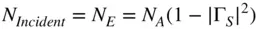

which is consistent with the definition of Eq. (1.47). Since the available noise at the output of a network doesn't depend upon the load impedance, the available gain from a network similarly doesn't depend upon the load impedance, and the available noise at the input of the network can be computed as Eq. (1.58), the measurement of noise figure defined in this way is not dependent upon the match of the noise receiver. One way to understand this is to note that the available gain is the maximum gain that can be delivered to a load. If the load is not conjugately matched to Γ 2, both the available gain and the available noise power at the output would be reduced by equal amounts, leaving the noise figure unchanged and independent of the noise receiver load impedance. Thus, for the case of noise measurements, the available noise power and available gain have been the important terms of use historically.