Joel P. Dunsmore - Handbook of Microwave Component Measurements
Здесь есть возможность читать онлайн «Joel P. Dunsmore - Handbook of Microwave Component Measurements» — ознакомительный отрывок электронной книги совершенно бесплатно, а после прочтения отрывка купить полную версию. В некоторых случаях можно слушать аудио, скачать через торрент в формате fb2 и присутствует краткое содержание. Жанр: unrecognised, на английском языке. Описание произведения, (предисловие) а так же отзывы посетителей доступны на портале библиотеки ЛибКат.

- Название:Handbook of Microwave Component Measurements
- Автор:
- Жанр:
- Год:неизвестен
- ISBN:нет данных
- Рейтинг книги:5 / 5. Голосов: 1
-
Избранное:Добавить в избранное
- Отзывы:
-
Ваша оценка:
Handbook of Microwave Component Measurements: краткое содержание, описание и аннотация
Предлагаем к чтению аннотацию, описание, краткое содержание или предисловие (зависит от того, что написал сам автор книги «Handbook of Microwave Component Measurements»). Если вы не нашли необходимую информацию о книге — напишите в комментариях, мы постараемся отыскать её.
Handbook of Microwave Component Measurements — читать онлайн ознакомительный отрывок
Ниже представлен текст книги, разбитый по страницам. Система сохранения места последней прочитанной страницы, позволяет с удобством читать онлайн бесплатно книгу «Handbook of Microwave Component Measurements», без необходимости каждый раз заново искать на чём Вы остановились. Поставьте закладку, и сможете в любой момент перейти на страницу, на которой закончили чтение.
Интервал:
Закладка:
which is substituted into Eq. (1.8)and Eq. (1.9), and from (1.15)one can directly compute a 1and b 1as
(1.23) 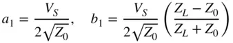
From here S 11can be derived from inspection as
(1.24) 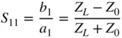
It is common to refer to S11 informally as the input impedance of the network, where
(1.25) 
This is clearly true for a 1‐port network and can be extended to a 2‐port or n‐port network if all the ports of the network are terminated in the reference impedance; but in general, one cannot say that S 11is the input impedance of a network without knowing the termination impedance of the network. This is a common mistake that is made with respect to determining the input impedance or S‐parameters of a network. S 11is defined for any terminations by Eq. (1.21), but it is the same as the input impedance of the network only under the condition that it is terminated in the reference impedance, thus satisfying the conditions for Eq. (1.20). Consider the network of Figure 1.2where the load is not the reference impedance; as such, it is noted that a 1and b 1exist, but now Γ 1(also called Γ Infor a 2‐port network) is defined as
(1.26) 
with the network terminated in an arbitrary impedance. As such, Γ 1represents the input impedance of a system comprised of the network and its terminating impedance. The important distinction is that S‐parameters of a network are invariant to the input of output terminations, providing they are defined to a consistent reference impedance, whereas the input impedance of a network depends upon the termination impedance at each of the other ports. The value of Γ 1of a 2‐port network can be directly computed from the S‐parameters and the terminating impedance, Z L, as
(1.27) 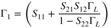
where Γ Lcomputed as in Eq. (1.24)is
(1.28) 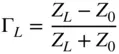
or in the case of a 2‐port network terminated by an arbitrary load then
(1.29) 
Similarly, the output impedance of a network that is sourced from an arbitrary source impedance is
(1.30) 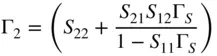
Another common term for the input impedance is the voltage standing wave ratio, called VSWR (also simply called SWR), and it represents the ratio of maximum voltage to minimum voltage that one would measure along a Z 0transmission line terminated in some arbitrary load impedance. It can be shown that this ratio can be defined in terms of the S‐parameters of the network as
(1.31) 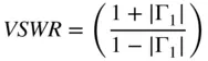
If the network is terminated in its reference impedance, then Γ 1becomes S 11. Another common term used to represent the input impedance is the reflection coefficient, ρ In, where
(1.32) 
It's also common to write
(1.33) 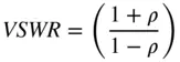
Another term related to the input impedance is return loss , which is alternatively defined as
(1.34) 
with the second definition being most properly correct, as loss is defined to be positive in the case where a reflected signal is smaller than the incident signal. But, in many cases, the former definition is more commonly used; the microwave engineer must simply refer to the context of the use to determine the proper meaning of the sign. Thus, an antenna with 14 dB return loss would be understood to have a reflection coefficient of 0.2, and the value displayed on a measurement instrument might read −14 dB.
For transmission measurements, the figure of merit is often gain or insertion loss (sometimes called isolation when the loss is very high). Typically this is expressed in dB, and similarly to return loss, it is often referred to as a positive number. Thus
(1.35) 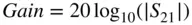
Insertion loss or isolation is defined as
(1.36) 
Again, the microwave engineer will need to use the context of the discussion to understand that a device with 40 dB isolation will show on an instrument display as −40 dB, due to the instrument using the evaluation of Eq. (1.35).
Notice that in the return loss, gain, and insertion loss equations, the dB value is given by the formula 20log 10(| S nm|), and this is often a source of confusion because common engineering use of dB has the computation as X dB= 10log 10( X ). This apparent inconsistency comes from the desire to have power gain when expressed in dB be equal to voltage gain, also expressed in dB. In a device sourced from a Z 0source and terminated in a Z 0load, the power gain is defined as the power delivered to the load relative to the power delivered from the source, and the gain is
(1.37) 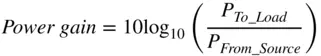
The power from the source is the incident power | a 1| 2, and the power delivered to the load is | b 2| 2. The S‐parameter gain is S 21and in a matched source and load situation is simply
(1.38) 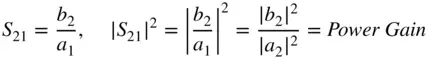
Интервал:
Закладка:
Похожие книги на «Handbook of Microwave Component Measurements»
Представляем Вашему вниманию похожие книги на «Handbook of Microwave Component Measurements» списком для выбора. Мы отобрали схожую по названию и смыслу литературу в надежде предоставить читателям больше вариантов отыскать новые, интересные, ещё непрочитанные произведения.


Обсуждение, отзывы о книге «Handbook of Microwave Component Measurements» и просто собственные мнения читателей. Оставьте ваши комментарии, напишите, что Вы думаете о произведении, его смысле или главных героях. Укажите что конкретно понравилось, а что нет, и почему Вы так считаете.