Mohammad Asadzadeh - An Introduction to the Finite Element Method for Differential Equations
Здесь есть возможность читать онлайн «Mohammad Asadzadeh - An Introduction to the Finite Element Method for Differential Equations» — ознакомительный отрывок электронной книги совершенно бесплатно, а после прочтения отрывка купить полную версию. В некоторых случаях можно слушать аудио, скачать через торрент в формате fb2 и присутствует краткое содержание. Жанр: unrecognised, на английском языке. Описание произведения, (предисловие) а так же отзывы посетителей доступны на портале библиотеки ЛибКат.
- Название:An Introduction to the Finite Element Method for Differential Equations
- Автор:
- Жанр:
- Год:неизвестен
- ISBN:нет данных
- Рейтинг книги:3 / 5. Голосов: 1
-
Избранное:Добавить в избранное
- Отзывы:
-
Ваша оценка:
An Introduction to the Finite Element Method for Differential Equations: краткое содержание, описание и аннотация
Предлагаем к чтению аннотацию, описание, краткое содержание или предисловие (зависит от того, что написал сам автор книги «An Introduction to the Finite Element Method for Differential Equations»). Если вы не нашли необходимую информацию о книге — напишите в комментариях, мы постараемся отыскать её.
An Introduction to the Finite Element Method (FEM) for Differential Equations
An Introduction to the Finite Element Method
An Introduction to the Finite Element Method for Differential Equations — читать онлайн ознакомительный отрывок
Ниже представлен текст книги, разбитый по страницам. Система сохранения места последней прочитанной страницы, позволяет с удобством читать онлайн бесплатно книгу «An Introduction to the Finite Element Method for Differential Equations», без необходимости каждый раз заново искать на чём Вы остановились. Поставьте закладку, и сможете в любой момент перейти на страницу, на которой закончили чтение.
Интервал:
Закладка:
The usual three types of boundary conditions.
1 Dirichlet boundary conditionHere, the solution is known at the boundary of the domain, asThis is the case, for example, describing a fixed temperature at the boundary.
2 Neumann boundary conditionIn this case, the derivative of the solution in certain direction is given:,where is, e.g. the outward unit normal to at and
3 Robin boundary condition (a combination of 1 and 2),In a homogeneous case, i.e. for , Robin condition means that the heat flux through the boundary is proportional to the temperature (in fact the temperature difference between the inside and outside) at the boundary.Example 1.8In two dimensions, with and hence, for , we have , see Figure 1.2. Figure 1.2Outward unit normal at a point .Example 1.9Let . We determine the normal derivative of in (the assumed normal) direction . The gradient of is the vector valued function , where and are the unit orthonormal basis in : and . Note that is not a unit vector. The normalized is obtained as , i.e.Thus, which givesThe usual three criteria to deal with1) In theoryA given differential equation problem is called well‐posed if the following three conditions hold true:I1. Existence: there exists at least one solution .I2. Uniqueness: we have either one solution or no solutions at all.I3. Stability: the solution depends continuously on the data.Note: A property that concerns behavior, such as growth or decay, or perturbations of a solution as time increases is generally called a stability property.2) In applicationsII1. Construction: exact design of the solution.II2. Regularity: how smooth is the found solution.II3. Approximation: when an exact construction is not possible.
Three general approaches for solving differential equations
1 Separation of variables method: The separation of variables technique reduces the (PDEs) to simpler EVPs (ODEs). This method is known as Fourier method, or solution by eigenfunction expansion.
2 Variational formulation method: Variational formulation or the multiplier method is a strategy for extracting information by multiplying a differential equation by suitable test functions and then integrating (e.g. like Fourier or Laplace transforms). This is also referred to as The Energy Method. A discrete version of this is the subject of our study.
3 Green's function method: Fundamental solutions, or solution of integral equations, which we have briefly addressed in the chapter of mathematical tools is the subject of an advanced PDE course.
1.3 PDEs in, Further Classifications
In this section, we extend the overture of the Sections 1.1and 1.2to higher dimensions and give definitions for linearity, nonlinearity, and superposition concepts.
We recall the common notation  for the real Euclidean spaces of dimension
  with the elements
  . In most of the applications,
  will be
  , or 4 and the variables
  denote coordinates in space dimensions, whereas
  represents the time variable. In this case, we usually replace
  by the most common notation:
  . Further, we shall use the subscript notation for the partial derivatives, viz.

A more general notation for partial derivatives of a sufficiently smooth function  (see Definition 1.1 below) is given by
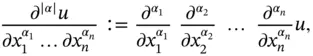
where 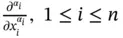 , denotes the partial derivative of order
  with respect to the variable
  , and
, and  is a multi‐index of integers
  with
with 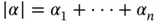 .
.
Definition 1.1
A function  of one real variable is said to be of class
  on an open interval
  if its derivatives
  exist and are continuous on
  . A function
  of
of  real variables is said to be of class
  on a set
  if all of its partial derivatives of order
  , i.e.
 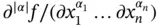 with the multi‐index
  and
and  , exist and are continuous on
  .
.
Интервал:
Закладка:
Похожие книги на «An Introduction to the Finite Element Method for Differential Equations»
Представляем Вашему вниманию похожие книги на «An Introduction to the Finite Element Method for Differential Equations» списком для выбора. Мы отобрали схожую по названию и смыслу литературу в надежде предоставить читателям больше вариантов отыскать новые, интересные, ещё непрочитанные произведения.


Обсуждение, отзывы о книге «An Introduction to the Finite Element Method for Differential Equations» и просто собственные мнения читателей. Оставьте ваши комментарии, напишите, что Вы думаете о произведении, его смысле или главных героях. Укажите что конкретно понравилось, а что нет, и почему Вы так считаете.