Mohammad Asadzadeh - An Introduction to the Finite Element Method for Differential Equations

These are some of the questions that we want to deal within this text when approximating with the FEMs.

A linear ODE of order has the general form:where denotes the derivative, with respect to , and , with (the ‐th order derivative). The corresponding linear differential operator is denoted by

Problems modeled by PDEs of the second order can be classified using, the so‐called, trinities. Below we introduce basic ingredients of this concept. For detailed study see, e.g. [68].

The usual three operators in PDEs of second order in .

(1.2.1)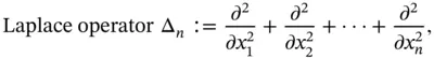

(1.2.2)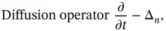

(1.2.3)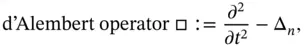

where we have the space variable , the time variable , and denotes the second partial derivative with respect to . We also define a first‐order operator, namely the gradient operator which is the vector valued operator

Often, the dimension is obvious from the context and therefore, usually, the subindex is suppressed and the operators and are simply denoted by (or by ) and , respectively.

Classifying general second‐order PDEs in two dimensions.

1 I) The constant coefficients caseA second‐order PDE in two dimensions, with constant coefficients, can be written in its general form asWe introduce the discriminant : a quantity that specifies the role of the coefficients of the second‐order terms, in determining the equation type in the sense that the equation isElliptic: if Parabolic: if and Hyperbolic: if Example 1.2Below are the classes of the most common, second‐order differential equations (in any dimension) and examples of their forms in :Potential equationHeat equationWave equation (elliptic) (parabolic) (hyperbolic).

2 II) The case of variable coefficientsIn the variable coefficients case, one can only have a local classification.Example 1.3Consider the Tricomi equation of gas dynamics:Here, the coefficient is not a constant, and we have and . Hence, and consequently, the domain of ellipticity is , and so on, see Figure 1.1. Figure 1.1Tricomi equation: an example of a variable coefficient classification.

The usual three types of problems in differential equations.

1 Initial value problems (IVPs)The simplest differential equation is for . But for any such , also for any constant . To determine a unique solution, a specification of the initial value is generally required. For example for , we have and the general solution is . With an initial value of , we get . Hence, the unique solution to this IVP is . Likewise, for a time‐dependent differential equation of second order (two time derivatives), the initial values for , i.e. and , are generally required. For a PDE such as the heat equation, the initial value can be a function of the space variable.Example 1.4The wave equation, on the real line, augmented with the given initial data:Remark 1.1Note that, here, for the unbounded spatial domain , it is required that (or =constant) as . This corresponds to two boundary conditions.

2 Boundary value problems (BVP)Example 1.5 (A BVP in )Consider the one‐dimensional stationary heat equation:In order to determine a solution uniquely (see Remark 1.2), the differential equation is complemented by boundary conditions imposed at the boundary points and ; for example and , where and are given real numbers.Example 1.6(A BVP in ).The Laplace equation in , Remark 1.2In general, in order to obtain a unique solution for a (partial) differential equation, one needs to supply physically adequate boundary data. For instance for the potential problem , stated in a rectangular domain , to determine a unique solution we need to give two boundary conditions in the ‐direction, i.e. the numerical values for and , and another two in the ‐direction: the numerical values of and . Whereas to determine a unique solution for the wave equation , it is necessary to supply two initial conditions in the time variable , and two boundary conditions in the space variable . We observe that in order to obtain a unique solution, we need to supply the same number of boundary (initial) conditions as the order of the differential equation in each spatial (time) variable. The general rule is that one should supply as many conditions as the highest order of the derivative in each variable. See also Remark 1.1, in the case of unbounded spatial domain.

3 Eigenvalue problems (EVPs)Let be a given square, say matrix. The relation , is a linear equation system, where is an eigenvalue and is an eigenvector. In the Example 1.7below, we introduce the corresponding terminology for differential equations. Example 1.7A differential equation describing a time‐independent vibrating string is given bywhere is an eigenvalue and is an eigenfunction. and are boundary values.To derive this equation, we consider the differential equation for a time‐dependent vibrating string, with small displacement , which is fixed at the end points, viz.Then, using the separation of variables technique, this equation is split into two EVPs: Insert (a nontrivial solution) into the differential equation to get(1.2.4) Dividing (1.2.4) by separates the variables so that we have(1.2.5) Consequently we get two ODEs (two EVPs):(1.2.6)