Mohammad Asadzadeh - An Introduction to the Finite Element Method for Differential Equations

Many colleagues have been involved in the design, presentation, and correction of the material in this book. I wish to thank Niklas Eriksson and Bengt Svensson who have read the entire manuscript and made many valuable suggestions. Niklas has contributed to a better presentation of the text as well as to simplifications and corrections of many key estimates that has substantially improved the quality of the book. Bengt has made all xfig figures. The final version is further polished by John Bondestam Malmberg and Tobias Gebäck who, in particular, have many useful input in the Matlab codes. Many others have been involved in teaching and/or assisting me in teaching whole or parts of the content of the book as well as helping in design of computer assignments. They have supplied invaluable feedback and raised the quality of this work. Here are some (far from all): Fredrik Benzon, Christoffer Cromvik, Tommy Gustafsson, Kristin Kirchner, Fredrik Lindgren, Anders Logg, Fardin Saedpanah, Christoffer Standar, Maximilian Thaller. I owe all of them and the un‐named supporting colleagues my most sincere gratitude.

Mohammad Asadzadeh

Göteborg, Sweden

August 2019

There are two ways of spreading light:

to be the candle or the mirror that reflects it.

Edith Wharton

This book presents an introduction to the Galerkin finite element method (FEM) as a powerful and general tool for approximating solution of differential equations. Our objective is twofold.

1 i) To present the main ordinary and partial differential equations (ODEs and PDEs) modeling different phenomena in science and engineering and introduce mathematical tools and environments for their analytic and numerical studies.

2 ii) To construct some common FEMs for approximate solutions of differential equations and analyze their well‐posedness (existence, uniqueness, and stability of such approximate solutions) as well as the accuracy of the approximation.

In its final step, a finite element procedure yields a linear system of equations (LSEs) where the unknowns are the approximate values of the solution at certain nodes. Then, an approximate solution is constructed by adapting piecewise polynomials of certain degree to these, approximate, nodal values.

The entries of the coefficient matrix and the right‐hand side of FEM's final LSEs consist of integrals which, e.g. for complex geometries or less smooth, and/or more complex, data, are not always easily computable. Therefore, numerical integration and quadrature rules are introduced to approximate such integrals. Furthermore, iteration procedures are included in order to efficiently compute the numerical solutions of such obtained LSEs.

Interpolation techniques are presented for both accurate polynomial approximations and also to derive basic a priori and a posteriori error estimates necessary to determine qualitative properties of the approximate solutions. That is to show how the approximate solution, in some adequate measuring environment, e.g. a certain norm, approaches the exact solution as the number of nodes, hence, the number of unknowns increases. For convenience, the frequently used classical inequalities, such as the Cauchy–Schwarz' and Poincare, likewise the inverse and trace estimates , that are of vital importance in error analysis and stability estimates, are introduced. In the theoretical abstraction, we demonstrate the fundamental solution approach based on Green's functions and prove the Riesz (Lax–Milgram) theorem which is essential in proving the existence of a unique solution for a minimization problem that in turn is equivalent both to a variational formulation as well as a corresponding boundary value problem (BVP).

Galerkin's method for solving a general differential equation is based on seeking an approximate solution, which is

1 Easy to differentiate and integrate

2 Spanned by a set of “nearly orthogonal” base functions in a finite‐dimensional vector space.

3 Satisfies Galerkin orthogonality relation.Roughly speaking, this means a closeness relation in the sense that:I). In a priori case, the difference between the exact and approximate solution is orthogonal to the finite dimensional vector space of the approximate solution.II). In a posteriori case, the residual of the approximate solution (=the difference between the left‐ and right‐hand side of an expression obtained from the differential equation where exact solution is replaced by the approximate solution) is orthogonal to the finite dimensional vector space of the approximate solution.

In this section, we give a brief introduction to some key concepts in differential equations. A standard classification and some general properties are presented in Trinities below.

A differential equation is a relation between an unknown function and its derivatives.

If the differentiation in the equation is with respect to only one variable, e.g. , (or in ), then the equation is called an ordinary differential equation (ODE).

As a simple example of an ODE, we mention the population dynamics model

(1.1.1)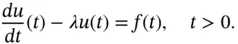

If , then the equation is called homogeneous ; otherwise, it is called inhomogeneous . For , the homogeneous equation 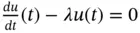has an exponentially growing analytic solution given by 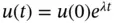, where is the initial population. On the contrary, yields a population that vanishes (dies out) with time.

The order of a differential equation is the order of the highest derivative of the function that appears in the equation.

If the function depends on more than one variable, and the differential equation possesses derivatives with respect to at least two variables, then the differential equation is called a partial differential equation (PDE), e.g.is a homogeneous PDE of the second order, whereas for , the equationsandare nonhomogeneous PDEs of the second order.

A solution to a differential equation is a function; (e.g. , , or above), which satisfies the corresponding differential equation.

In general, the solution of a differential equation cannot be expressed in terms of elementary functions, and numerical methods are the only way to solve the differential equations through constructing approximate solutions. Then, the main questions areTo what extent does the approximate solution preserve the physical properties of the exact solution, or satisfies a corresponding, discrete, version of the differential equation (consistency)?How sensitive is the solution to the change of the data (stability)?How close is the approximate solution to the exact solution (convergence)?Which are the adequate environments to measure this closeness?