Mohammad Asadzadeh - An Introduction to the Finite Element Method for Differential Equations

(1.5.11)

Here, , called the specific heat , is assumed to be constant. Next, we relate the temperature to the heat flux . Here, we use Fourier's law but, first, to be specific, we describe the simple facts supporting Fourier's law:

1 i. Heat flows from regions of high temperature to regions of low temperature.

2 ii. The rate of heat flux is small or large accordingly as temperature changes between neighboring regions are small or large.

To describe these quantitative properties of heat flux, we postulate a linear relationship between the rate of heat flux and the rate of temperature change. Recall that if is a point in the heat‐conducting medium and is a unit vector specifying a direction at , then the rate of heat flow at in the direction is and the rate of change of the temperature is , the directional derivative of the temperature. Since requires , and vice versa (from calculus the direction of maximal growth of a function is given by its gradient), our linear relation takes the form , with . Since specifies any direction at , this is equivalent to the assumption

(1.5.12)

which is Fourier's law . The positive function is called the heat conduction (or Fourier) coefficient . Let now and and insert ( 1.5.11) and ( 1.5.12) into ( 1.5.10) to get the final form of the heat equation:

(1.5.13)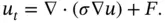

The quantity is referred to as the thermal diffusivity (or diffusion) coefficient . If we assume that is constant, then the final form of the heat equation would be

(1.5.14)

The third equation in ( 1.5.2) is the wave equation: 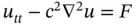. Here, represents a wave traveling through an ‐dimensional medium; is the speed of propagation of the wave in the medium and is the amplitude of the wave at position and time . The wave equation provides a mathematical model for a number of problems involving different physical processes as, e.g. in the following examples (i)–(vi):

1 (i) Vibration of a stretched string, such as a violin string (one‐dimensional).

2 (ii)Vibration of a column of air, such as a clarinet (one‐dimensional).

3 (iii)Vibration of a stretched membrane, such as a drumhead (two‐dimensional).

4 (iv)Waves in an incompressible fluid, such as water (two‐dimensional).

5 (v)Sound waves in air or other elastic media (three‐dimensional).

6 (vi)Electromagnetic waves, such as light waves and radio waves (three‐dimensional).

Note that in (i), (iii) and (iv), represents the transverse displacement of the string, membrane, or fluid surface; in (ii) and (v), represents the longitudinal displacement of the air; and in (vi), is any of the components of the electromagnetic field. For detailed discussions and a derivation of the equations modeling (i)–(vi), see, e.g. Folland [62], Strauss [129], and Taylor [134]. We should point out, however, that in most cases, the derivation involves making some simplifying assumptions. Hence, the wave equation gives only an approximate description of the actual physical process, and the validity of the approximation will depend on whether certain physical conditions are satisfied. For instance, in example (i), the vibration should be small enough so that the string is not stretched beyond its limits of elasticity. In example (vi), it follows from Maxwell's equations, the fundamental equations of electromagnetism, that the wave equation is satisfied exactly in regions containing no electrical charges or current, which of course cannot be guaranteed under normal physical circumstances and can only be approximately justified in the real world. So an attempt to derive the wave equation corresponding to each of these examples from physical principles is beyond the scope of these notes. Nevertheless, to give an idea, below we shall derive the wave equation for a vibrating string.