Dario Grana - Seismic Reservoir Modeling

The probability P ( a < X ≤ b , c < Y ≤ d ) of X and Y being in the domain ( a , b ] × ( c , d ] is defined as the double integral of the joint PDF:

(1.21)

Given the joint distribution of X and Y , we can compute the marginal distributions of X and Y , respectively, as:

(1.22)

(1.23)

In the multivariate setting, we can also introduce the definition of conditional probability distribution. For continuous random variables, the conditional PDF of X ∣ Y is:

(1.24)

where the joint distribution f X,Y( x , y ) is normalized by the marginal distribution f Y( y ) of the conditioning variable. An analogous definition can be derived for the conditional distribution f Y∣X( y ) of Y ∣ X . All the definitions in this section can be extended to any finite number of random variables.

An example of joint and conditional distributions in a bivariate domain is shown in Figure 1.4. The surface plot in Figure 1.4shows the bivariate joint distribution f X,Y( x , y ) of two random variables X and Y centered at (1, −1). The contour plot in Figure 1.4shows the probability density contours of the bivariate joint distribution as well as the conditional distribution f Y∣X( y ) for the conditioning value x = 1 and the marginal distributions f X( x ) and f Y( y ).

The conditional probability distribution in Eq. (1.24)can also be computed using Bayes' theorem ( Eq. 1.8) as:

(1.25)

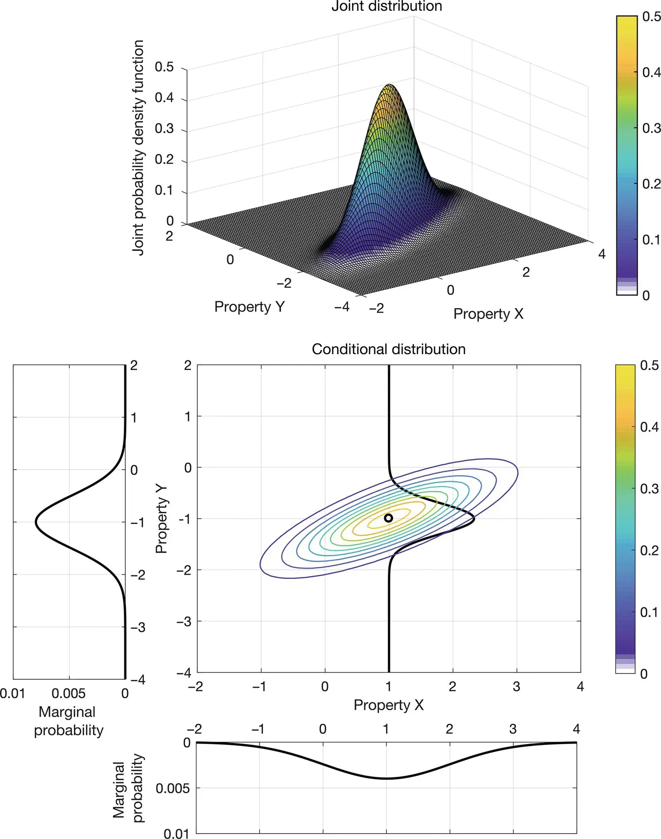
Figure 1.4Multivariate probability density functions: bivariate joint distribution (surface and contour plots), conditional distribution for x = 1, and marginal distributions.

Figure 1.5shows an example where the uncertainty in the prior probability distribution of a property X is relatively large, and it is reduced in the posterior probability distribution of the property X conditioned on the property Y , by integrating the information from the data contained in the likelihood function. In seismic reservoir characterization, the variable X could represent S‐wave velocity and the variable Y could represent P‐wave velocity. If a direct measurement of P‐wave velocity is available, we can compute the posterior probability distribution of S‐wave velocity conditioned on the P‐wave velocity measurement. The prior distribution is assumed to be unimodal with relatively large variance. By integrating the likelihood function, we reduce the uncertainty in the posterior distribution.

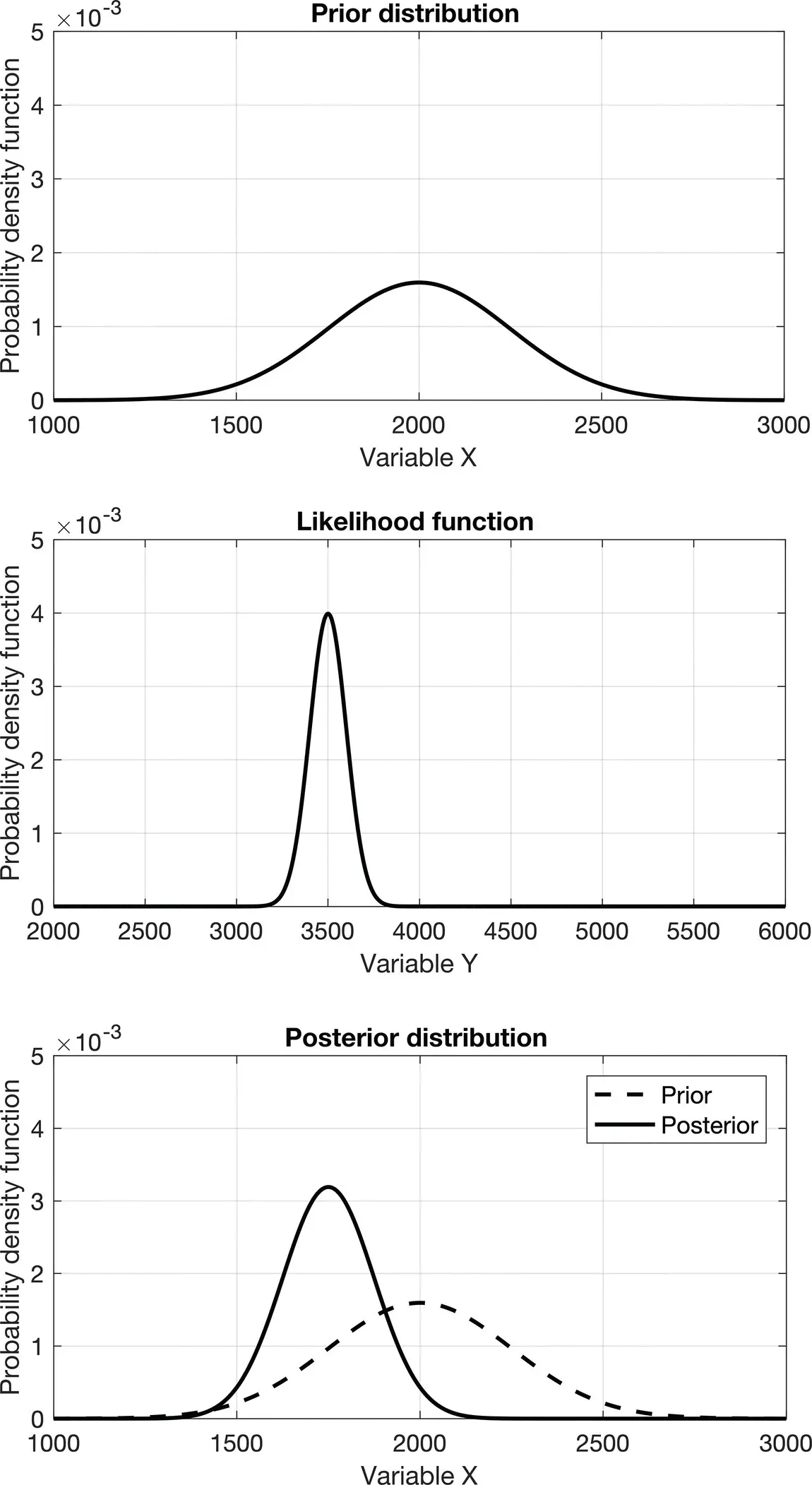
Figure 1.5Bayes' theorem: the posterior probability is proportional to the product of the prior probability and the likelihood function.

We can also extend the definitions of mean and variance to multivariate random variables. For the joint distribution f X,Y( x , y ) of X and Y , the mean μ X,Y= [ μ X, μ Y] Tis the vector of the means μ Xand μ Yof the random variables X and Y . In the multivariate case, however, the variances of the random variables do not fully describe the variability of the joint random variable. Indeed, the variability of the joint random variable also depends on how the two variables are related. We define then the covariance σ X,Yof X and Y as:

(1.26)

The covariance is a measure of the linear dependence between two random variables. The covariance of a random variable with itself is equal to the variance of the variable. Therefore, and . The information associated with the variability of the joint random variable is generally summarized in the covariance matrix ∑ X,Y:

(1.27)

where the diagonal of the matrix includes the variances of the random variables, and the elements outside the diagonal represent the covariances. The covariance matrix is symmetric by definition, because σ X,Y= σ Y,Xbased on the commutative property of the multiplication under the integral in Eq. (1.26). The covariance matrix of a multivariate probability distribution is always positive semi‐definite; and it is positive definite unless one variable is a linear transformation of another variable.

We then introduce the linear correlation coefficient ρ X,Yof two random variables X and Y , which is defined as the covariance normalized by the product of the standard deviations of the two random variables:

(1.28)

The correlation coefficient is by definition bounded between −1 and 1 (i.e. −1 ≤ ρ X,Y≤ 1), dimensionless, and easy to interpret. Indeed, a correlation coefficient ρ X,Y= 0 means that X and Y are linearly uncorrelated, whereas a correlation coefficient | ρ X,Y| = 1 means that Y is a linear function of X . Figure 1.6shows four examples of two random variables X and Y with different correlation coefficients. When the correlation coefficient is ρ X,Y= 0.9, the samples of the two random variables form an elongated cloud of points aligned along a straight line, whereas, when the correlation coefficient is ρ X,Y≈ 0, the samples of the two random variables form a homogeneous cloud of points with no preferential alignment. A positive correlation coefficient means that if the random variable X increases, then the random variable Y increases as well, whereas a negative correlation coefficient means that if the random variable X increases, then the random variable Y decreases. For this reason, when the correlation coefficient is ρ X,Y= −0.6, the cloud of samples of the two random variables approximately follows a straight line with negative slope.