Dario Grana - Seismic Reservoir Modeling

We first discuss discrete random variables and then generalize to continuous random variables. A discrete random variable is a variable that can only take a finite number of values (i.e. values in a set N of finite cardinality). For example, tossing a coin or rolling a die are examples of experiments involving discrete random variables. When tossing a coin, the outcome of the random variable is either heads or tails, whereas, when rolling a die, the outcome is a positive integer from 1 to 6. Facies, flow units, or rock types are examples of discrete random variables in subsurface modeling. These variables are often called categorical random variables to indicate that the outcomes of the random variable have no intrinsic order.

Although the outcome of a discrete random variable is uncertain, we can generally assess the probability of each outcome. In other words, we can define the probability of a discrete random variable X by introducing a function p X: N → [0, 1], where the probability P ( x ) of an outcome x is given by the value of the function p X, i.e. P ( x ) = p X( X = x ). The uppercase symbol generally represents the random variable, whereas the lowercase symbol represents the specific outcome. The function p Xis called probability mass function and it has the following properties:

(1.10)

for all outcomes x ∈ N ; and

(1.11)

Equations (1.10)and (1.11)imply that the probability of each outcome is a real number in the interval [0, 1] and that the sum of the probabilities of all the possible outcomes is 1. The probability mass function p Xis generally represented by a histogram (or a bar chart for categorical variables).

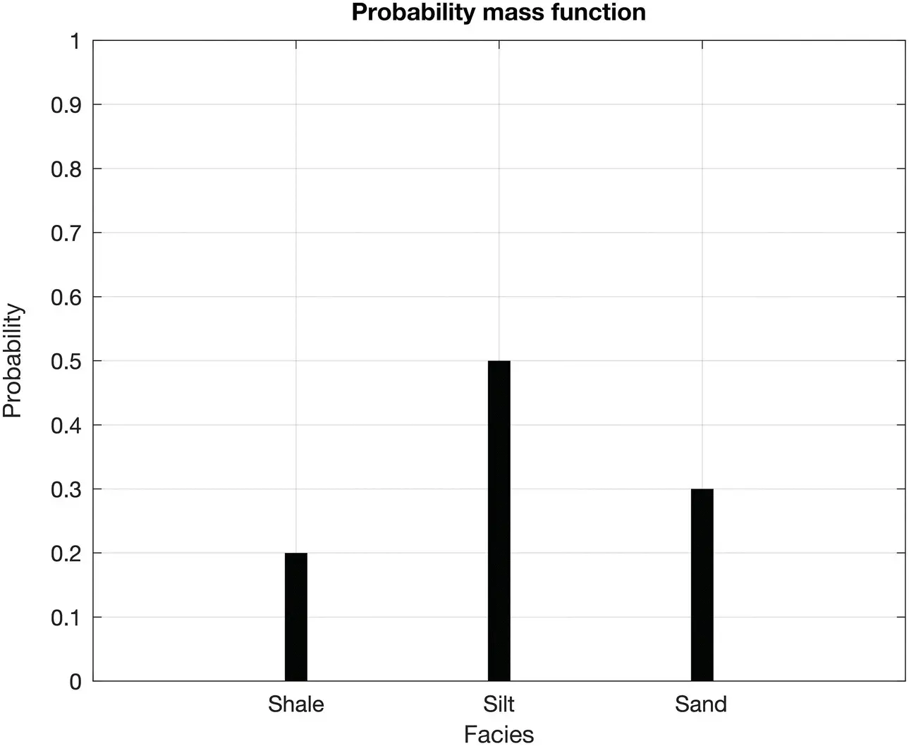
For example, if we roll a die, there are only six possible outcomes, and the probability of each outcome for a fair die is P ( X = i ) = 1/6, for i = 1, …, 6. In a reservoir model where three facies have been identified, for example sand, silt, and shale, the probability mass function is represented by the bar chart of the facies proportions, i.e. the normalized frequency of the facies. In Example 1.1, the prior probabilities of the facies are P ( A = shale ) = 0.2; P ( A = silt ) = 0.5; P ( A = sand ) = 0.3. These probabilities form the probability mass function of the facies and can be represented by a bar chart, as in Figure 1.1.

In the continuous case, the probability of a continuous random variable X is defined by introducing a non‐negative integrable function f X: ℝ → [0, +∞]. The function f Xis called probability density function (PDF) and must satisfy the following properties:

(1.12)

(1.13)

(1.14)

Equations (1.12)– (1.14)imply that the likelihood of each outcome is a real number in the interval [0, +∞] and that the integral of the PDF in the domain of X is 1. Because a continuous variable can take infinitely many values, there is an infinite number of possible outcomes; therefore, the probability that a continuous variable X takes the exact value x is 0, i.e. P ( X = x ) = 0. For this reason, instead of computing the probability of an exact value x , we define the probability of the outcome x to belong to a subset of the domain of the random variable X .

Figure 1.1Bar chart of the probability mass function of a discrete random variable representing the reservoir facies in Example 1.1.

The PDF f X( x ) is then used to define the probability of a subset of values of the random variable X . We define the probability of the outcome x being in the interval ( a , b ] as the definite integral of the PDF in the interval ( a , b ]:

(1.15)

The interval ( a , b ] can be infinitesimally small or it can extend to ±∞. For example, we can study the probability P (0.20 < ϕ ≤ 0.21) of porosity ϕ being between 0.20 and 0.21 or the probability P ( V P> 5.5) of P‐wave velocity V Pbeing greater than 5.5 km/s. The graphical interpretation of the definition of probability in Eq. (1.15)is shown in Figure 1.2, where the curve represents the PDF of the random variable X , and the area delimited by the PDF and the x ‐axis of the graph between a = 2 and b = 3, i.e. the definite integral of the curve in the interval (2, 3], represents the probability P (2 < X ≤ 3).

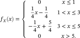
In this example, we illustrate the calculation of the probability of the random variable X to belong to the interval (2, 3], assuming that X is distributed according to the triangular PDF shown in Figure 1.2. The random variable in Figure 1.2could represent, for example, the P‐wave velocity of a porous rock, expressed in km/s.

The PDF f X( x ) can be written as follows:

The triangular function f X( x ) is a non‐negative function with integral equal to 1 (i.e. the area of the triangle with base of length 4 and height 0.5); hence, it satisfies the conditions in Eqs. (1.12)– (1.14), and it is a valid PDF. We now compute the probability P (2 < X ≤ 3) using the definition in Eq. (1.15):

The probability P (2 < X ≤ 3) represents the area of the region highlighted in Figure 1.2and can also be computed as the area of a right trapezoid, rotated by 90°.

In many applications, it is useful to describe the distribution of the continuous random variable using the concept of cumulative distribution function (CDF), F X: ℝ → [0, 1]. We assume that a random variable X has a PDF f X( x ); then, the CDF F X( x ) is defined as the integral of f X( x ) in the interval (−∞, x ]: