Dario Grana - Seismic Reservoir Modeling

If two random variables are independent, i.e. f X,Y( x , y ) = f X( x ) f Y( y ), then X and Y are uncorrelated. However, the opposite is not necessarily true. Indeed, the correlation coefficient is a measure of linear correlation; therefore, if two random variables are uncorrelated, then there is no linear relation between the two properties, but it does not necessarily mean that the two variables are independent. For example, if Y = X 2, and X takes positive and negative values, then the correlation coefficient is close to 0, but yet Y depends deterministically on X through the quadratic relation ( Figure 1.6), and the two variables are not independent.

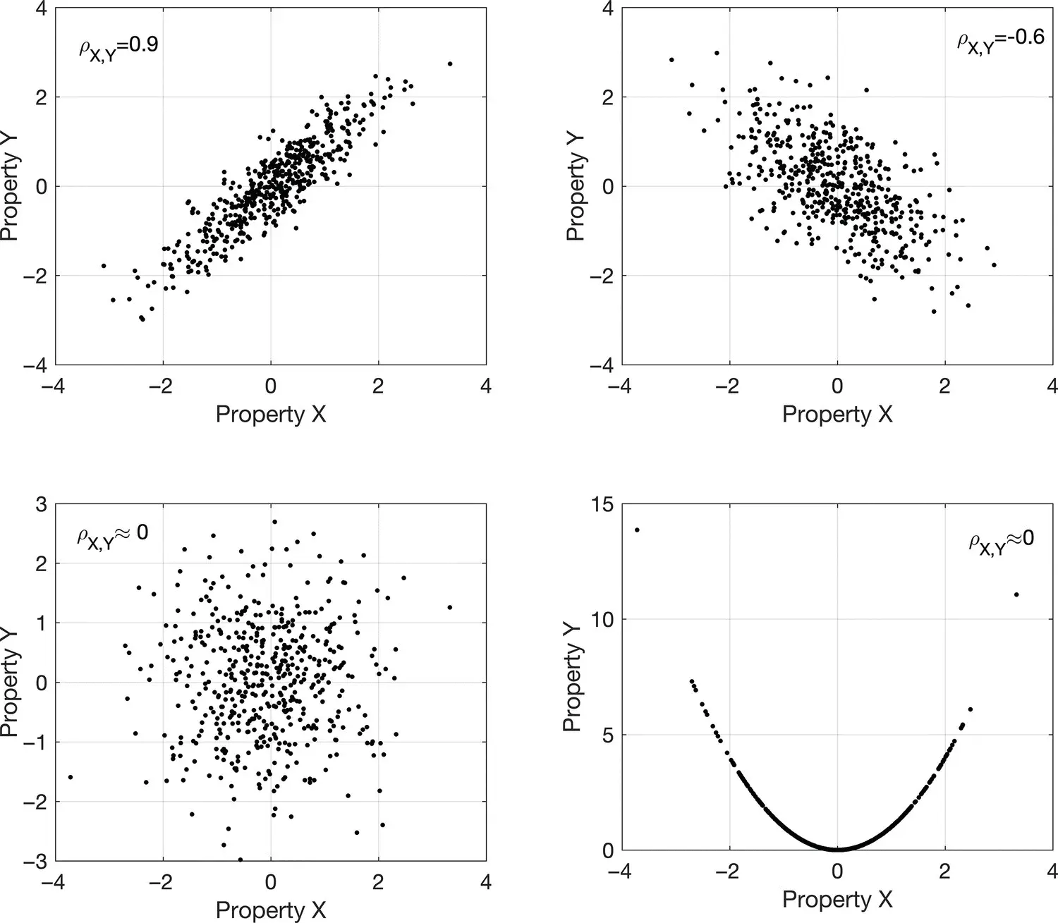
Figure 1.6Examples of different correlations of the joint distribution of two random variables X and Y . The correlation coefficient ρ X,Yis 0.9 and −0.6 in the top plots and approximately 0 in the bottom plots.

Different probability mass and density functions can be used for discrete and continuous random variables, respectively. For parametric distributions, the function is completely defined by a limited number of parameters (e.g. mean and variance). In this section, we review the most common probability mass and density functions. Probability mass functions are commonly used in geoscience problems for discrete random variables such as facies or rock types, whereas PDFs are used for continuous properties such as porosity, fluid saturations, density, P‐wave and S‐wave velocity. Some applications in earth sciences include mixed discrete–continuous problems with both discrete and continuous random variables.

The simplest probability distribution is the Bernoulli distribution and it is associated with a single experiment with only two possible outcomes. An example of this type of experiment is the toss of a coin. Let X be a random variable representing the experiment, then X is a random variable that takes only two outcomes, 0 and 1, where X = 1 means that a favorable event is observed, and X = 0 otherwise. We assume that the probability of the favorable event, generally called the probability of success, is a real number p such that 0 ≤ p ≤ 1. The probability mass function p X( x ) is then:

(1.29)

The mean of the Bernoulli distribution is then μ X= p and the variance is .

The Bernoulli distribution has several applications in earth sciences. In reservoir modeling, for example, we can use the Bernoulli distribution for the occurrence of a given facies or rock type. For instance, we define a successful event as finding a high‐porosity sand rather than impermeable shale. The probability of success is generally unknown and it depends on the overall proportions of the two facies.

A common distribution for discrete and continuous properties is the uniform distribution on a given interval. According to a uniform distribution, a random variable is equally likely to take any value in the assigned interval. Hence, the PDF is constant within the interval, and 0 elsewhere. If a random variable X is distributed according to a uniform distribution U ([ a , b ]) in the interval [ a , b ], then its PDF f X( x ) can be written as:

(1.30)

The mean μ Xof a uniform distribution in the interval [ a , b ] is:

(1.31)

and it coincides with the median, whereas the variance is:

(1.32)

An example of uniform distribution in the interval [1, 3] is shown in Figure 1.7. The uniform distribution is sometimes called non‐informative because it does not provide any additional knowledge other than the interval boundaries.

Most of the random variables of interest in reservoir modeling are continuous. The most common PDF for continuous variables is the Gaussian distribution, commonly called normal distribution. We say that a random variable X is distributed according to a Gaussian distribution with mean μ Xand variance , if its PDF f X( x ) can be written as:

(1.33)

A Gaussian distribution with 0 mean and variance equal to 1 is also called standard Gaussian distribution (or normal distribution). The Gaussian distribution is symmetric and unimodal ( Figure 1.8) and can be used to describe a number of phenomena in nature. The Gaussian distribution is defined on the entire set ℝ of real numbers and it is always positive. For example, the standard Gaussian distribution in Figure 1.8is always greater than 0, but the probability of the random variable being greater than 3 or less than 3 is close to 0, hence negligible.

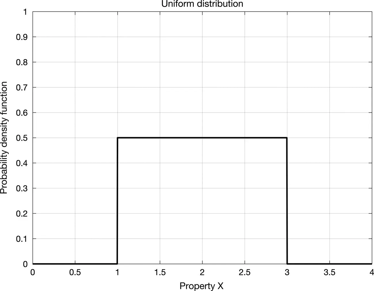
Figure 1.7Uniform probability density function in the interval [1, 3].

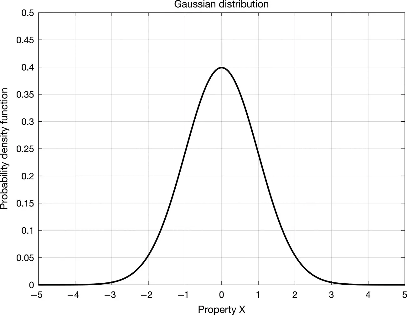
Figure 1.8Standard Gaussian probability density function with 0 mean and variance equal to 1.

As shown in Eq. (1.15), in order to compute any probability associated with the random variable X , we must compute an integral. For a Gaussian distribution, the integral of Eq. (1.33)has no analytical form; therefore, we must use numerical tables of the cumulative density function of the standard Gaussian distribution (Papoulis and Pillai 2002). For example, if X is a random variable distributed according to a standard Gaussian distribution , then we can compute the following probabilities P ( X ≤ 1) ≅ 0.84, P ( X ≤ 1.5) ≅ 0.932, P ( X ≤ 2) ≅ 0.977, using the numerical tables. Similarly, we obtain that P (−1 ≤ X ≤ 1) ≅ 0.68, P (−2 ≤ X ≤ 2) ≅ 0.954, and P (−3 ≤ X ≤ 3) ≅ 0.997.