Dario Grana - Seismic Reservoir Modeling

We say that a random variable X is distributed according to a Gaussian mixture distribution of n components, if the PDF f X( x ) can be written as:

(1.40)

where the distributions represent the Gaussian components with mean μ X∣kand variance , and the coefficients πk are the weights of the linear combination with the condition . The condition on the sum of the weights guarantees that f X( x ) is a valid PDF.

Figure 1.10shows an example of Gaussian mixture PDF with two components with weights equal to 0.4 and 0.6, means equal to −2 and 2, and equal variance of 1. The resulting PDF is multimodal owing to the presence of two components with different mean values and asymmetric due to the larger weight of the second component.

An example of bivariate Gaussian mixture distribution with two components is shown in Figure 1.11. The PDF in Figure 1.11is estimated from a geophysical dataset of porosity and P‐wave velocity. The two components represent two different rock types, namely high‐porosity sand and impermeable shale. The mean of porosity in the sand component is 0.22, whereas the mean of porosity in shale is 0.06. Porosity and P‐wave velocity are negatively correlated in both components; however, the Gaussian mixture distribution shows a larger variance within the sand component, probably because of the rock heterogeneity and the fluid effect. The distribution is truncated for porosity less than 0, to avoid non‐physical values.

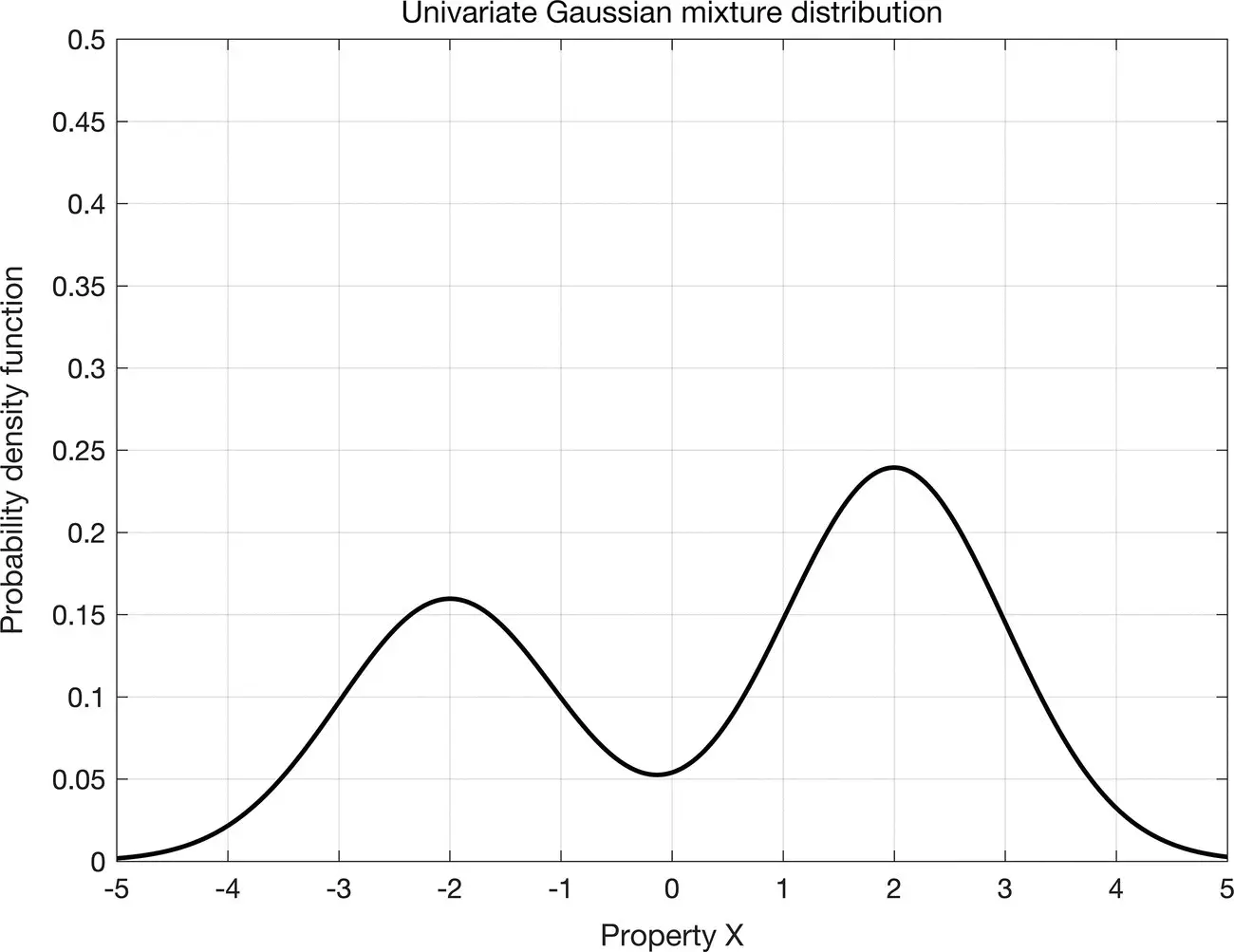
Figure 1.10Univariate Gaussian mixture probability density function, with two components with weights equal to 0.4 and 0.6, means equal to −2 and 2, and equal variance of 1.

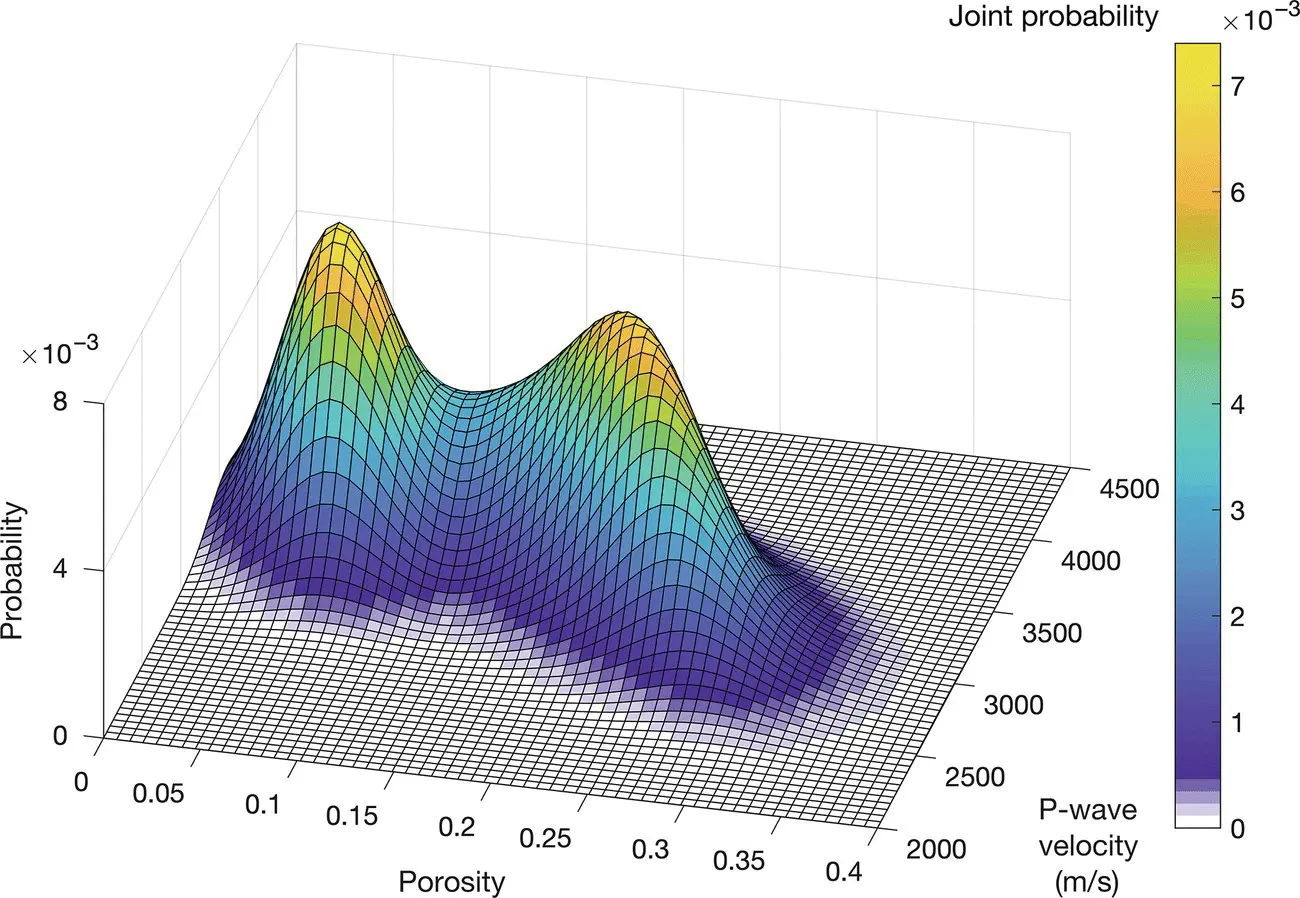
Figure 1.11Bivariate Gaussian mixture probability density function estimated from a geophysical dataset, in the porosity–velocity domain.

The Beta distribution is a PDF for continuous random variables defined in the interval [0, 1]. The PDF is uniquely defined by two positive parameters, namely α and β , that determine the shape of the distribution and its derivatives. The generalization to the multivariate domain is the Dirichlet distribution.

A random variable X is distributed according to a Beta distribution B ( X ; α , β ) with parameters α > 0 and β > 0, in the interval [0, 1], if its PDF f X( x ) can be written as:

(1.41)

where the denominator is a normalizing constant to ensure that Eq. (1.41)is a valid PDF (i.e. the integral of the PDF is equal to 1). The mean μ Xof a Beta distribution is:

(1.42)

whereas the variance is:

(1.43)

The Beta distribution is a suitable model for random variables describing volumetric fractions, since it is defined on the interval [0, 1]; however, it is not commonly used in practical applications owing to the limited analytical tractability. In geoscience applications, it is often convenient to use the Beta PDF as a prior distribution in Monte Carlo sampling algorithms to sample bounded random variables such as fluid saturations. Figure 1.12shows two examples of Beta distributions with parameters α = β = 0.1 (convex curve, solid line) and α = β = 2 (concave curve, dashed line) that could be used to describe the distribution of fluid saturations and mineral fractions in a hydrocarbon reservoir, respectively. The convex distribution in Figure 1.12shows high likelihood for values near the boundaries of the interval [0, 1], and low likelihood in the middle of the interval. This behavior is often observed in fluid saturations in the subsurface, where partial saturations are unlikely owing to the gravity effect. The concave distribution in Figure 1.12shows low likelihood for values near the boundaries of the interval [0, 1], and high likelihood in the middle of the interval. This behavior is often observed in mineral fractions in the subsurface, where rocks are generally made of mixtures of minerals rather than pure minerals.

In some applications, we might be interested in transformations of random variables, or, in other words, in the response of a function of a random variable. For example, in reservoir modeling, we might be interested in the permeability distribution, and because of the lack of direct measurements, we estimate the distribution as a function of the distribution of another random variable, for example, porosity.

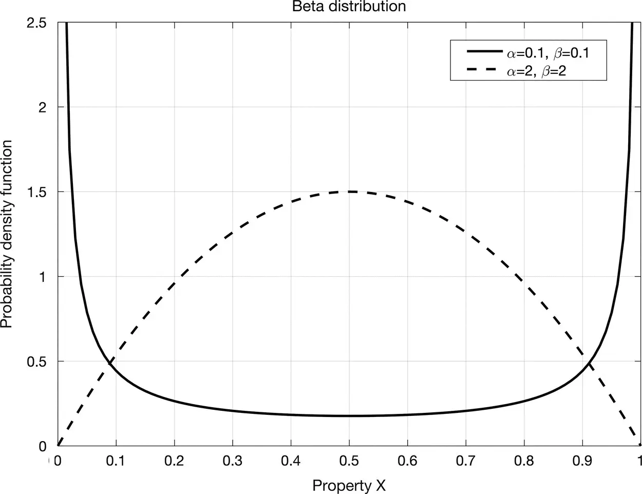
Figure 1.12Beta probability density function in the interval [0, 1]: the solid line (convex curve) represents a Beta distribution with parameters α = β = 0.1, whereas the dashed line (concave curve) represents a Beta distribution with parameters α = β = 2.

If the transformation is linear, then the shape of the distribution of the linear response is the same as the distribution of the initial random variable. For example, if the distribution of the initial random variable is Gaussian, then the distribution of the predicted random variable is also Gaussian. As shown in Section 1.4.3, a Gaussian distribution is fully described by its mean and variance; therefore, to compute the PDF of the transformed variable, we simply compute the mean and the variance of the transformed distribution.

For example, if X is distributed according to a Gaussian distribution with mean μ Xand variance , and we apply a linear transformation Y = g ( X ) = aX + b , then Y is still distributed according to a Gaussian distribution with mean μ Y: