Dario Grana - Seismic Reservoir Modeling

To compute a probability associated with a non‐standard Gaussian distribution with mean μ Yand variance , we apply the transformation X = ( Y − μ Y)/ σ Yand we use the numerical tables of the standard Gaussian distribution. Indeed, the random variable X is a standard Gaussian distribution with 0 mean and variance equal to 1, and For example, if Y has a Gaussian distribution with mean μ Y= 1 and variance , then we define a new random variable X = ( Y − 1)/2. The probability P ( Y ≤ 2) is then equal to the probability P ( X ≤ 0.5) ≅ 0.69. Similarly, P (−3 ≤ Y ≤ 3) = P (−2 ≤ X ≤ 1) ≅ 0.82.

In general, the probability that a Gaussian random variable X takes values in the interval ( μ X− σ X, μ X+ σ X) is approximately 0.68; in the interval ( μ X− 2 σ X, μ X+ 2 σ X) is approximately 0.95; and in the interval ( μ X− 3 σ X, μ X+ 3 σ X) is approximately 0.99. Therefore, there is a high probability that the values of the Gaussian random variable are in the interval of length 6 σ Xcentered around the mean μ X, even though the tails of the distributions have non‐zero probability for values greater than μ X+ 3 σ Xor less than μ X− 3 σ X.

Because a Gaussian PDF takes positive values in the entire real domain, when using Gaussian distributions for bounded random variables, such as volumetric fractions, or positive random variables, such as velocities, one should truncate the distribution to avoid non‐physical outcomes or apply a suitable transformation (Papoulis and Pillai 2002), such as the normal score or logit transformations of the original variables.

We then introduce the log‐Gaussian distribution (or log‐normal distribution) that is strictly related to the Gaussian distribution. Log‐Gaussian distributions are commonly used for positive random variables. For example, suppose that we are interested in the probability distribution of P‐wave velocity. To avoid positive values of the PDF for negative (hence non‐physical) P‐wave velocity values, we can take the logarithm of P‐wave velocity and assume a Gaussian distribution in the logarithmic domain. In this case, the distribution of P‐wave velocity is said to be log‐Gaussian.

We say that a random variable Y is distributed according to a log‐Gaussian distribution with mean μ Yand variance , if X = log( Y ) is distributed according to a Gaussian distribution . The PDF f Y( y ) can be written as:

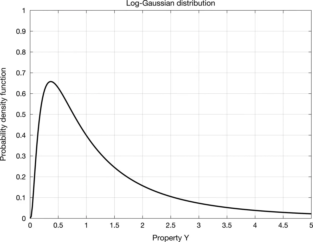
Figure 1.9Log‐Gaussian probability density function associated with the standard Gaussian distribution in Figure 1.8.

(1.34)

where μ Xand are the mean and the variance of the random variable in the logarithmic domain.

The mean μ Yand the variance of the log‐Gaussian distribution are related to the mean μ Xand variance of the associated Gaussian distribution, according to the following transformations:

(1.35)

(1.36)

(1.37)

(1.38)

Figure 1.9shows the log‐Gaussian distribution associated with the standard Gaussian distribution shown in Figure 1.8.

A log‐Gaussian distributed random variable takes only positive real values. Its distribution is unimodal but it is not symmetric since the PDF is skewed toward 0. The skewness s of a log‐Gaussian distribution is always positive and is given by:

(1.39)

For these reasons, the log‐Gaussian distribution is a convenient and useful model to describe unimodal positive random variables in earth sciences.

An example of application of log‐Gaussian distributions in seismic reservoir characterization can be found in Section 5.3, where we assume a multivariate log‐Gaussian distribution of elastic properties in the Bayesian linearized seismic inversion.

Gaussian and log‐Gaussian distributions are unimodal parametric distributions. However, many rock properties in the subsurface, for example porosity and permeability, are multimodal. Multimodal distributions can be described by non‐parametric distributions, but these distributions require a large amount of data to be estimated. In many applications, multimodal distributions can be approximated by Gaussian mixture distributions, i.e. linear combinations of Gaussian distributions.