Fundamentals of Terahertz Devices and Applications

Using Love's Equivalence Principle, the electric fields computed at the aperture plane ( z = h ) can be used to compute the equivalent magnetic and electric currents outside of the surface where is the normal vector to the aperture surface, in this case , and and are the electric fields computed at the aperture plane using the full‐wave simulator. The use of a full‐wave simulator will provide the accuracy to obtain the fields on an aperture grid, which will allow the computation of the currents using the free space Green's function and the equivalence principle. The infinite silicon medium can be simulated by setting absorbing boundaries in the full‐wave simulator. An electric field probe is set on the air‐silicon interface and will be the origin of our primary field origin of coordinates xyz (the plane is marked in red in Figure 2.15).

The lens can be in the radiative near field or far field of the feed. In the case of the leaky‐wave feed, due to its high directivity, the lens will be in most cases in the radiative near field. In the radiative region of the near‐field, the field can still be represented by a local spherical wave with an angular distribution that depends on the distance, and therefore the same PO explained previously can still be used. The near and far‐field effect is illustrated in Figure 2.16, where the fields are computed over a sphere of two certain radius ρ = 4.5 λ and ρ = 20 λ . The far field is calculated independently of the lens geometry, as the dependency in r is eliminated (i.e. the term e −jkr/ r ). This dependency is added when the equivalent currents are computed over the lens. From the phase shown in the radiation patterns, we can see that the phase center is not in the plane of the iris ground plane, as shown in Figure 2.15, it is below and it varies with frequency. Thus, in the contrary to the design equations on the previous sections, the lens extension height L and radius R will need adjustment to maximize the aperture efficiency of the overall antenna. This aperture efficiency will be computed over an aperture of diameter D (see Fig. 2.17a), which is smaller than the lens radius R because of the high directivity of the leaky‐wave feed.

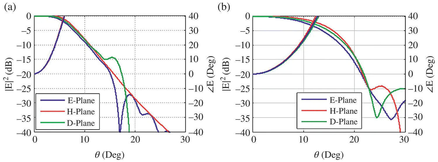
Figure 2.16Amplitude and phase of the electric centered at a central frequency 550 GHz in the (a) far‐field and (b) near‐field at ρ = 4.5 λ of the leaky‐wave feed radiating over an infinite silicon medium.

This part will cover the design of a leaky‐wave feed with an integrated silicon lens in the order of 4 − 20 λ as described in [33]. We will start by choosing a leaky‐wave feed that is matched over 15% bandwidth and provides the highest directivity by using a resonant Fabry–Perot air‐cavity. For a desired aperture diameter, the procedure to design the overall integrated silicon lens dimensions, shown in Figure 2.17a is, as follows:

1 The waveguide, iris, and air cavity are optimized at the central frequency. After setting the air cavity thickness to λ0/2,the other dimensions of the waveguide and iris can be optimized with a full‐wave simulator for maximum radiation efficiency. The dimensions and reflection coefficient are shown in Figure 2.14for a central frequency of 550 GHz. Next, the electric field components in the aperture plane are exported from the 3D simulator in order to perform the optimization of the lens geometry using the formulation previously explained. Figure 2.17(a) Drawing of the basic parameters of the shallow lens antenna geometry. (b) Taper angle θf as a function of ρ for a shallow lens of diameter D = 2.5 mm and D = 5 mm, calculated at the central frequency of 550 GHz. Figure 2.18Optimum (a) taper angle θf and (b) lens thickness W as a function of each diameter D that maximize the lens antenna performance using the procedure described.

2 Obtain the basic dimensions W and taper edge angle θf. From the exported fields we will compute the radiated field from the leaky‐wave feed inside the infinite silicon for different ρ. After this, we will calculate the taper edge angle θf for a certain taper field value in the 10–14 dB region. The field taper is chosen according to the tradeoff between the spillover and the taper efficiency, equivalent to the tradeoff in reflector antennas. This computation of the field at different ρ is necessary because, for the dimension of the lens aperture, the feed is placed on the near field of the antenna. This dependency can be seen in Figure 2.17b, when we move toward the far‐field region this dependency fades, and the curves in Figure 2.17b get flatten (θf becomes a constant with ρ). The optimal ρ and θf value will be given by the intersection of this curve with . Figure 2.18a shows the optimal ρ and θf values for different diameters ranging from 4 − 11λ0. And Figure 2.18b shows the optimum distance W defined as where the shallow lens surface should be placed.

3 The shallow lens surface is optimized to maximize the antenna directivity. The lens curvature is defined by the radius R and the height H, or equivalently by the extension height L (see Figure 2.19a). For planar antennas, the optimum L and R are known, see Section 2.3. However, as stated previously, because the phase center of the leaky wave is below the waveguide aperture, this makes the optimum lens surface differ from the standard cases [33]. Then, we will vary the height and radius of the lens until the optimum is achieved. The variation of the directivity as a function of the extension height L is shown in Figure 2.18b. To perform this optimization, full‐wave simulators are not recommended as the computational time and complexity of the global structure is considerably. Instead, the PO techniques described previously provide a good compromise between quality of the results and computational time which makes it fundamental for integration into optimization of lenses. The optimum at different field tapers for each diameter are summarized in Figure 2.20a and b. Figure 2.19(a) The shallow lens of diameter D is defined by a corresponding H and R. (b) Taper and aperture efficiency as a function of the lens extension height L.

4 Following these two steps, we can obtain the highest directivity for a desired aperture diameter D for the designed leaky‐wave feed. The directivity attainable with this architecture is shown in Figure 2.21a. Note that for the chosen field tapers of −10 dB to −14 dB the spillover remains below 0.25 dB. The Gaussicity, calculated with the expressions on Section II is shown in Figure 2.21b. The beamwaist and the phase center of the lens have been adjusted to maximized the Gaussicity for each diameter. As it is shown very high Gaussicity values can be achieved across all the diameters due to the high symmetry and shape of the leaky‐wave field.

The main advantage of having a lens antenna with a waveguide feed is its seamless integration in an array configuration for waveguide‐based receivers at submillimeter‐wave frequencies. As explained in previous sections, the leaky‐wave feed illuminates a small aperture of diameter D of the lens, making the resulting effective lens surface a very shallow lens. These shallow lenses can be packed together forming an array and it can be fabricated using silicon micromachining techniques. The feed and lens array can be entirely fabricated over a few silicon wafers and stacked to the rest of the instrument (see Figure 2.22).