Stephen Rolt - Optical Engineering Science

(4.29)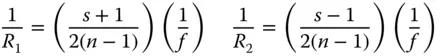

Figure 4.10illustrates the lens shape parameter for a series of lenses with positive focal power. For a symmetric, bi-convex lens, the shape factor is zero. In the case of a plano-convex lens, the shape factor is 1 where the plane surface faces the image and is −1 where the plane surface faces the object. A shape factor of greater than 1 or less than −1 corresponds to a meniscus lens. Here, both radii have the same sense, i.e. they are either both positive or both negative. For a shape parameter of greater than 1, the surface with the greater curvature faces the object and for a shape parameter of less than −1, the surface with the greater curvature faces the image. Of course, this applies to lenses with positive power. For (diverging) lenses with negative power, then the sign of the shape factor is opposite to that described here.

Having parameterised the object and image distances and the lens radii in terms of the conjugate parameter, shape parameter, and lens power, we can recast the expressions in Eqs. (4.25a)– (4.25d)in a more generic form. With a little algebraic manipulation, we obtain the following expressions for the Gauss-Seidel aberration of a lens with the stop at the lens surface:

(4.30a)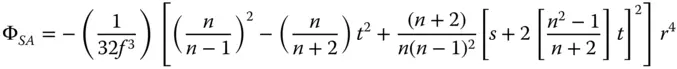

(4.30b)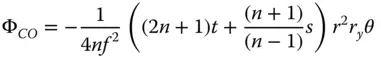

(4.30c)

(4.30d)

Again, casting all expressions in the form set out in Chapter 3, as for the expressions for the mirror we have

(4.31a)

(4.31b)

(4.31c)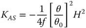

(4.31d)

Once again, the Petzval curvature is simply given by subtracting twice the K ASterm in Eq. (4.31c)from the field curvature term in Eq. (4.31d). This gives:

(4.32)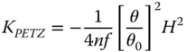

That is to say, a single lens will produce a Petzval surface whose radius of curvature is equal to the lens focal length multiplied by its refractive index. Once again, the Petzval sum may be invoked to give the Petzval curvature for a system of lenses:

(4.33)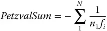

It is important here to re-iterate the fact that for a system of lenses, it is impossible to eliminate Petzval curvature where all lenses have positive focal lengths. For a system with positive focal power, i.e. with a positive effective focal length, there must be some elements with negative power if one wishes to ‘flatten the field’.

Before considering the aberration behaviour of simple lenses in a little more detail, it is worth reflecting on some attributes of the formulae in Eqs. (4.30a)– (4.30d). Both spherical aberration and coma are dependent upon the lens shape and conjugate parameters. In the case of spherical aberration there are second order terms present for both shape and conjugate parameters, whereas the behaviour for coma is linear. However, the important point to recognise is that the field curvature and astigmatism are independent of both lens shape and conjugate parameter and only depend upon the lens power. Once again, it must be emphasised that this analysis applies only to the situation where the stop is situated at the lens.

We will now look at a simple special case to apply to a thin lens with the stop at the lens. This is the common situation where a lens is being used to focus an object located at the infinite conjugate, such as a telescope objective or a lens focusing a parallel laser beam. From Eq. (4.26), the conjugate parameter, t , is equal to −1. Substituting t = −1 into Eq. (4.31a)gives the spherical aberration as:

(4.34)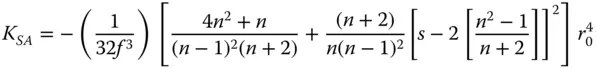

The important point to note about Eq. (4.34)is that the spherical aberration can never be equal to zero and that for a positive lens, K SAis always negative. This means that the longitudinal aberration for a positive lens is also negative and that, for all single lenses, more marginal rays are brought to a focus closer to the lens. Whilst Eq. (4.34)asserts that the spherical aberration in this case can never be zero, its magnitude can be minimised for a specific lens shape. Inspection of Eq. (4.34)reveals that this condition is met where:

(4.35)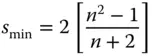

This optimum shape factor corresponds to the so-called ‘ best form singlet’ and is generally available from optical component suppliers, particularly with regard to applications in the focusing of laser beams. For a refractive index of 1.5, the optimum shape factor is around 0.7. This is close in shape to a plano-convex lens. However, it is important to emphasise, that optimum focusing is obtained where the more steeply curved surface is facing the infinite conjugate. Generally, also, where a plano-convex lens is used to focus a collimated beam, the curved surface should face the infinite conjugate. This behaviour is shown in Figure 4.11, which emphasises the quadratic dependence of spherical aberration on lens shape factor.

Coma for the infinite conjugate also depends upon the shape factor. However, in this instance, the dependence is linear. Once more, substituting t = −1 into Eq. (4.31b), we get:

(4.36)

Unlike in the case for spherical aberration, there exists a shape factor for which the coma is zero. This is simply given by: