Stephen Rolt - Optical Engineering Science

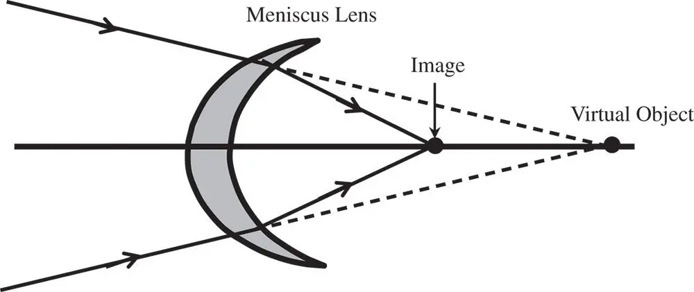
Figure 4.14 Aplanatic meniscus lens.

We now wish to add some power to the microscope objective hyperhemisphere set out in Worked Example 4.1. We are to do so with an extra meniscus lens situated at the vertex of the hyperhemisphere with a negligible separation. As with the hyperhemisphere, the meniscus lens is in the aplanatic arrangement. The meniscus lens is made of the same material as the hyperhemisphere, that is with a refractive index of 1.6. All properties of the hyperhemisphere are as set out in Worked Example 4.1.

What are the radii of curvature of the meniscus lens and what is the location of the (virtual) image for the combined system? The system is as illustrated below.

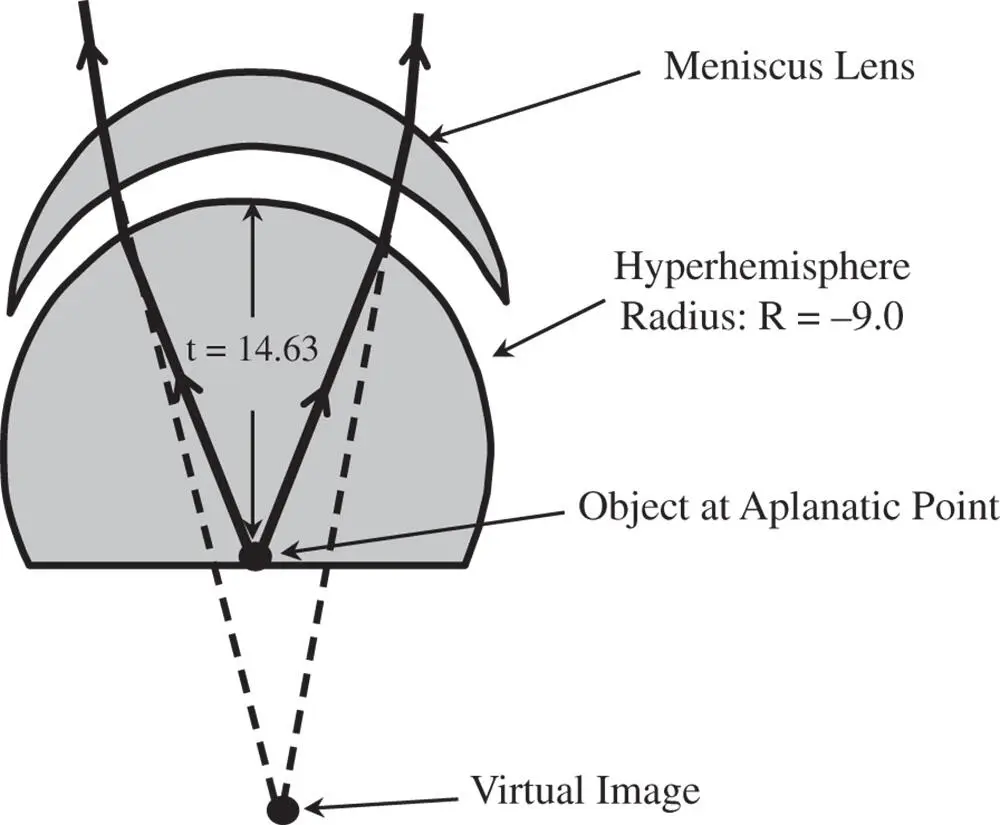
We know from Worked Example 4.1that the original image distance produced by the hyperhemisphere is −23.4 mm. The object distance for the meniscus lens is thus 23.4 mm. From Eq. (4.39a)we have:

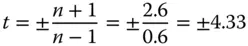
There remains the question of the choice of the sign for the conjugate parameter. If one refers to Figure 4.14, it is clear that the sense of the object and image location is reversed. In this case, therefore, the value of t is equal to +4.33 and the numerical aperture of the system is reduced by a factor of 1.6 (the refractive index). In that case, the image distance must be equal to minus 1.6 times the object distance. That is to say:

We can calculate the focal length of the lens from:

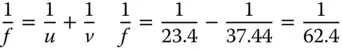
Therefore the focal length of the meniscus lens is 62.4 mm. If the conjugate parameter is +4.33, then the shape factor must be −(2n + 1), or −4.2 (note the sign). It is a simple matter to calculate the radii of the two surfaces from Eq. (4.29):

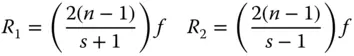
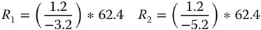
Finally, this gives R 1as − 23.4 mmand R 2as − 14.4 mm. The signs should be noted. This follows the convention that positive displacement follows the direction from object to image space.

If the microscope objective is ultimately to provide a collimated output – i.e. with the image at the infinite conjugate, the remainder of the optics must have a focal length of 37.44 mm (i.e. 23.4 × 1.6). This exercise illustrates the utility of relatively simple building blocks in more complex optical designs. This revised system has a focal length of 9 mm. However, the ‘remainder’ optics have a focal length of 37.4 mm, or only a quarter of the overall system power. Spherical aberration increases as the fourth power of the numerical aperture, so the ‘slower’ ‘remainder’ will intrinsically give rise to much less aberration and, as a consequence, much easier to design. The hyperhemisphere and meniscus lens combination confer much greater optical power to the system without any penalty in terms of spherical aberration and coma. Of course, in practice, the picture is complicated by chromatic aberration caused by variations in refractive properties of optical materials with wavelength. Nevertheless, the underlying principles outlined are very useful.

In all previous analysis, it is assumed that the stop is located at the optical surface in question. This is a useful starting proposition. However, in practice, this is most usually not the case. With the stop located at a spherical surface, by definition, the chief ray will pass directly through the vertex of that surface. If, however, the surface is at some distance from the stop, then the chief ray will, in general, intersect the surface at some displacement from the surface vertex. This displacement is, in the first approximation, proportional to the field angle of the object in question. The general concept is illustrated in Figure 4.15.

Instead of the stop being located at the surface in question, the stop is displaced by a distance, s, from the surface. The chief ray, passing through the centre of the stop defines the field angle, θ. In addition, the pupil co-ordinates defined at the stop are denoted by r xand r y. However, if the stop were located at the optical surface, then the field angle would be θ′, as opposed to θ. In addition, the pupil co-ordinates would be given by r x ′ and r y ′ . Computing the revised third order aberrations proceeds upon the following lines. All the previous analysis, e.g. as per Eqs. (4.31a)– (4.31d), has enabled us to express all aberrations as an OPD in terms of θ′, r x ′ , and r y ′ . It is clear that to calculate the aberrations for the new stop locations, one must do so in terms of the new parameters θ, r x, and r y. This is done by effecting a simple linear transformation between the two sets of parameters. Referring to Figure 4.15, it is easy to see:

(4.40a)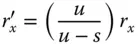

(4.40b)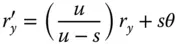

Figure 4.15 Impact of stop movement.

(4.40c)

The effective size of the pupil at the optic is magnified by a quantity M pand the pupil offset set out in Eq. (4.40b)is directly related to the eccentricity parameter, E, described in Chapter 2. Indeed, the product of the eccentricity parameter and the Lagrange invariant, H is simply equal to the ratio of the marginal and chief ray height at the pupil. That is to say:

(4.41)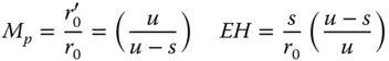

In this case, r 0refers to the pupil radius at the stop and r 0′ to the effective pupil radius at the surface in question. As a consequence, we can re-cast all three equations in a more convenient form.