Stephen Rolt - Optical Engineering Science

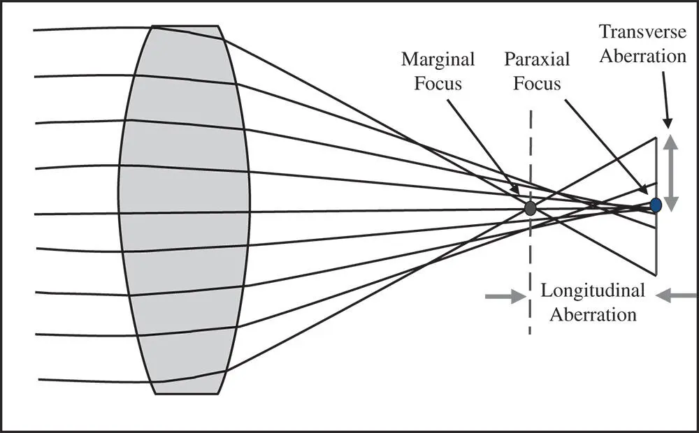
Figure 3.2 Transverse and longitudinal aberration.

(3.5)

In fact, if the radius of the pupil aperture is r 0and the lens focal length is f , then the longitudinal and transverse aberration are related in the following way:

(3.6)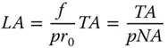

NA is the numerical aperture of the lens .

A plot of the transverse aberration against the pupil function is referred to as a ‘ ray fan’. Ray fans are widely used to provide a simple description of the fidelity of optical systems. If one views the transverse aberration at the paraxial focus, then the transverse aberration should show a purely cubic dependence upon the pupil function. This is illustrated in Figure 3.3a which shows the aberrated ray fan. If, one the other hand, the transverse aberration is plotted away from the paraxial focus, then an additional linear term is present in the plot. This is because pure defocus (i.e. without third order aberration) produces a transverse aberration that is linear with respect to pupil function. This is illustrated in Figure 3.3b which shows a ray fan where both the linear defocus and third order aberration terms are present.

The underlying amount of third order aberration is the same in both plots. However, the overall transverse aberration in Figure 3.3b (plotted on the same scale) is significantly lower than that seen in Figure 3.3a. This is because defocus can, to some extent, be used to ‘balance’ the original third order aberration. As a result, by moving away from the paraxial focus, the size of the blurred spot is reduced. In fact, there is a point at which the size (root mean square radius) of the spot is minimised. This optimum focal position is referred to as the circle of least confusion. This is illustrated in Figure 3.4.

Most generally, the transverse aberration where third order aberration is combined with defocus can be represented as:

(3.7)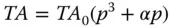

TA 0 is the nominal third order aberration and α represents the defocus

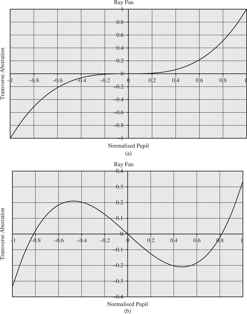
Figure 3.3 (a) Ray fan for pure third order aberration. (b) Ray fan with third order aberration and defocus.

Since the geometry is assumed to be circular, to calculate the rms (root mean square) aberration, one must introduce a weighting factor that is proportional to the pupil function, p . The mean squared transverse aberration is thus:

(3.8)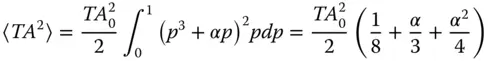

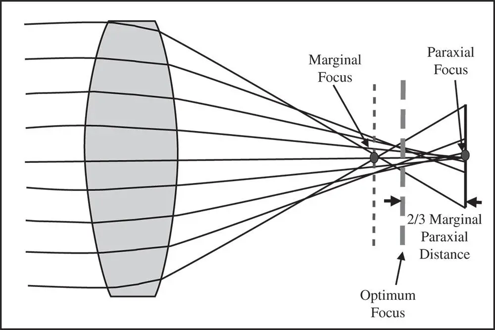
Figure 3.4 Balancing defocus against aberration – optimal focal position.

The expression is minimised where α = −2/3. To understand the significance of this, examination of Eq. (3.6)suggests that, without defocus, the marginal ray ( p = 1) has a longitudinal aberration of TA 0/ NA . The defocus term itself produces a constant longitudinal aberration or defocus of α TA 0/ NA . Therefore, the optimum defocus is equivalent to placing the adjusted focus at 2/3 of the distance between the paraxial and marginal focus, as shown in Figure 3.4. Without this focus adjustment, with the third order aberration viewed at the paraxial focus, the rms aberration is TA 0/4. However, adding the optimum defocus reduces the rms aberration to TA 0/12, a reduction by a factor of 3.

This analysis provides a very simple introduction to the concept of third order aberrations. In the basic illustration so far considered, we have looked at the example of a simple lens focussing an on axis object located at infinity. In the more general description of monochromatic aberrations that we will come to, this simple, on-axis aberration is referred to as spherical aberration. In developing a more general treatment of aberration in the next sections we will introduce the concept of optical path difference (OPD).

In the preceding section, we considered the impact of optical imperfections on the transverse aberration and the construction of ray fans. Unfortunately, this treatment, whilst providing a simple introduction, does not lead to a coherent, generalised description of aberration. At this point, we introduce the concept of optical path difference(OPD). For a perfect imaging system, with no aberration, if all rays converge onto the paraxial focus, then all ray paths must have the same optical path length from object to image. This is simply a statement of Fermat's principle. We now consider an aberrated system where we accurately ( not relying on the paraxial approximation ) trace all rays through the system from object to image. However, at the last surface, we ( hypothetically ) force all rays to converge onto the paraxial focus. For all rays, we compute the optical path from object to image. The OPD is the difference between the integrated optical path of a specified ray with respect to the optical path of the chief ray. Of course, if there were no aberration present, the OPD would be zero. Thus, the OPD represents a quantitative description of the violation of Fermat's principle.

The general concept is shown in Figure 3.5. Rays are accurately traced from the object through the system, emerging into image space. That is to say, ray tracing proceeds until the last optical surface, mirror or lens etc. Following the preceding discussion, at some point, we force all rays to converge upon the paraxial focus. However, the convention for computing OPD is that all rays are traced back to a spherical surface centred on the paraxial focus and which lies at the exit pupil of the system. Of course, it must be emphasised that the real rays do not actually follow this path. In the generic system illustrated, the real ray is traced to point P located in object space and the optical path length computed. Thereafter, instead of tracing the real ray into the object space, a dummy ray is traced, as shown by the dotted line. This dummy ray is traced from point P to point Q that lies on the reference surface – a sphere located at the exit pupil and centred on the paraxial focus. The optical path length of this segment is then added to the total.

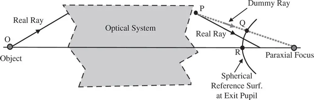
Figure 3.5 Illustration of optical path difference.

After calculating the optical path length for the dummy ray OPQ, we need to calculate the OPD with respect to the chief ray. The chief ray path is calculated from the object to its intersection with the reference sphere at the pupil, represented, in this instance, by the path OR. In calculating the OPD, the convention is that the OPD is the chief ray optical path (OR) minus the dummy ray optical path (OPQ). Note the sign convention.