Stephen Rolt - Optical Engineering Science

1 Haija, A.I., Numan, M.Z., and Freeman, W.L. (2018). Concise Optics: Concepts, Examples and Problems. Boca Raton: CRC Press. ISBN: 978-1-1381-0702-1.

2 Hecht, E. (2017). Optics, 5e. Harlow: Pearson Education. ISBN: 978-0-1339-7722-6.

3 Keating, M.P. (1988). Geometric, Physical, and Visual Optics. Boston: Butterworths. ISBN: 978-0-7506-7262-7.

4 Kidger, M.J. (2001). Fundamental Optical Design. Bellingham: SPIE. ISBN: 0-81943915-0.

5 Kloos, G. (2007). Matrix Methods for Optical Layout. Bellingham: SPIE. ISBN: 978-0-8194-6780-5.

6 Longhurst, R.S. (1973). Geometrical and Physical Optics, 3e. London: Longmans. ISBN: 0-582-44099-8.

7 Smith, F.G. and Thompson, J.H. (1989). Optics, 2e. New York: Wiley. ISBN: 0-471-91538-1.

In the first two chapters, we have been primarily concerned with an idealised representation of geometrical optics involving perfect or Gaussian imaging. This treatment relies upon the paraxial approximation where all rays present a negligible angle with respect to the optical axis. In this situation, all primary optical ray behaviour, such as refraction, reflection, and beam propagation, can be represented in terms of a series of linear relationships involving ray heights and angles. The inevitable consequence of this paraxial approximation and the resultant linear algebra is apparently perfect image formation. However, for significant ray angles, this approximation breaks down and imperfect image formation, or aberration, results. That is to say, a bundle of rays emanating from a single point in object space does not uniquely converge on a single point in image space.

This chapter will focus on monochromatic aberrationsonly. These aberrations occur where there is departure from ideal paraxial behaviour at a single wavelength. In addition, chromatic aberrationcan also occur where first order paraxial properties of a system, such as focal length and cardinal point locations, vary with wavelength. This is generally caused by dispersion, or the variation in the refractive index of a material with wavelength. Chromatic aberration will be considered in the next chapter.

A simple scenario is illustrated in Figure 3.1where a bundle of rays originating from an object located at the infinite conjugate is imaged by a lens. Figure 3.1a presents the situation for perfect imaging and Figure 3.1b illustrates the impact of aberration.

In Figure 3.1b, those rays that are close to the axis are brought to a focus at the paraxial focus. This is the ideal focus. However, those rays that are further from the axis are brought to a focus at a point closer to the lens than the paraxial focus. In fact, the behaviour illustrated in Figure 3.1b is representative of a simple lens; marginal rays are brought to a focus closer to the lens than the chief ray. However, in general terms, the sense of the aberration could be either positive or negative, with the marginal rays coming to a focus either before or after the paraxial focus.

In formulating perfect or Gaussian imaging we assumed all relationships are linear. For example, Snell's law of refraction was reduced in the following way:

(3.1)

In making the paraxial approximation, we are considering just the first or linear term in the Taylor series. The next logical stage in the process is to consider higher order terms in the Taylor series.

(3.2)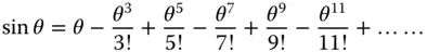

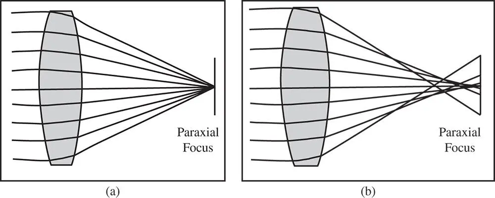
Figure 3.1 (a) Gaussian imaging. (b) Impact of aberration.

Following the term that is linear in θ, we have terms that are cubic or third order in θ. Of course, these third order terms are followed by fifth and seventh order terms etc. in succession. Third order aberration theorydeals exclusively with those imperfections associated with the third order departure from ideal behaviour, as illustrated in Eq. (3.2). Much of classical aberration theory is restricted to consideration of these third order terms and is, in effect a refinement or successive approximation to paraxial theory. Higher order (≥5) terms can be important in practical design scenarios. However, these are generally dealt with by numerical computation, rather than by a simple generically applicable theory.

Third order aberration theory forms the basis of the classical treatment of monochromatic aberrations. Unless specific steps are taken to correct third order aberrations in optical systems, then third order behaviour dominates. That is to say, error terms in the ray height or angle (compared to the paraxial) have a cubic dependence upon the angle or height. As a simple illustration of this, Figure 3.1b shows rays originating from a single object (at the infinite conjugate). For perfect image formation, the height of all rays at the paraxial focus should be zero, as in Figure 3.1a. However, the consequence of third order aberration is that the ray height at the paraxial focus is proportional to the third power of the original ray height (at the lens).

In dealing with third order aberrations, the location of the entrance pupil is important. Let us assume, in the example set out in Figure 3.1b, that the pupil is at the lens. If the radius of the entrance pupil is r 0and the height a specific ray at this point is h , then we may define a new parameter, the normalised pupil co-ordinate, p , in the following way:

(3.3)

The normalised pupil co-ordinate can have values ranging from −1 to +1, with the extremes representing the marginal ray. The chief ray corresponds to p = 0. At this stage, it is useful to provide a specific and quantifiable definition of aberration. The quantity, transverse aberration, is defined as the difference in height of a specific ray and the corresponding chief ray as measured at the paraxial focus. The ‘corresponding chief ray’ emanates from the same object point as the ray under consideration. In addition, the term longitudinal aberrationis also used to describe aberration. Longitudinal aberration (LA) is the axial distance from the point at which the ray in question intersects the chief ray and the location of the paraxial focus. The transverse aberration (TA) and longitudinal aberration definitions are illustrated in Figure 3.2.

In keeping with the previous arguments, the TA has a third order dependence upon the pupil function. This is illustrated in Eq. (3.4):

(3.4)

Transverse aberration has dimensions of length, whereas the pupil function is a dimensionless ratio. Geometrically, the LA is approximately equal to the transverse aberration divided by the ray angle which itself is proportional to the pupil function. Therefore, the longitudinal aberration has a quadratic dependence upon the pupil function. This is illustrated in Eq. (3.5).