Stephen Rolt - Optical Engineering Science

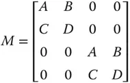
In this two dimensional representation, the matrix element representing each optical element would be a 4 × 4 matrix instead of a 2 × 2 matrix. However, the matrix is not fully populated in any realistic scenario. For a rotationally symmetric optical system, as we have been considering thus far, there can only be four elements:

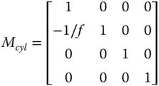
That is to say, the impact of each optical surface is identical in both the x and y directions in this instance. However, there are optical components where the behaviour is different in the x and y directions. An example of this might be a cylindrical lens,whose curvature in just one dimension produces focusing only in one direction. The two dimensional matrix for a cylindrical lens would look as follows:

A component that possesses different paraxial properties in the two dimensions is said to be anamorphic. A more general description of an anamorphic element is illustrated next:

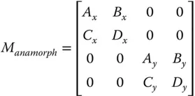
Note there are no non-zero elements connecting ray properties in different dimensions, x and y. This would require the surfaces produce some form of skew behaviour and this is not consistent with ideal paraxial behaviour. Since this is the case, the two orthogonal components, x and y, can be separated out and presented as two sets of 2 × 2 matrices and analysed as previously set out. All relevant optical properties, cardinal points are then calculated separately for x and y components. Even if focal points are identical for the two dimensions, the principal planes may not be co-located. This gives rise to different focal lengths for the x and y dimension and potentially differential image magnification. This differential magnification is referred to as anamorphic magnification. Significantly, in a system possessing anamorphic optical properties, the exit pupil may not be co-located in the two dimensions.

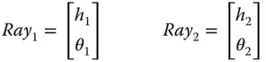
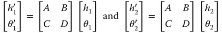
The field angle, i.e. the angle of the chief ray and the marginal ray angles, will change as the rays propagate through an optical system. The relationship between these angles is inherently constrained by the magnification properties of the optical system in the paraxial approximation. The optical invariantis a parameter that, in the paraxial approximation, constrains the relationship between any two rays that propagate through an optical system. We now have two general rays as described by their ray vectors:

The optical invariant, O, is given by:

(2.4)

The optical invariant is, in the paraxial approximation, preserved on passage through an optical system. That is to say:

(2.5)

n′ , h′ , θ′ , etc. are ray parameters following propagation .

Derivation of the above invariant is straightforward using matrix analysis.

Hence:

From (1.23) we know that the determinant of the matrix is given by the ratio of the refractive indices in the relevant media, so:

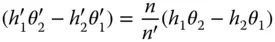
Finally we arrive at Eq. (2.5)

The optical invariant is a generalised constraint that relates system lateral and angular magnification and applies to any arbitrary pair of rays. A very specific descriptor is created when the ray pair consists of the chief ray and the marginal ray. This special case of the optical invariant is known as the Lagrange invariant. The Lagrange invariant, H is given by:

(2.6)

If we now simply evaluate H at the entrance and exit pupils where, by definition, h chiefis zero, then the product nh marginalθ chiefis constant. The Lagrange invariant then simply articulates the fact that the angular and lateral magnifications are inversely related. In fact, the Lagrange invariant captures a more fundamental constraint to an optical system. If the object plane is uniformly illuminated, then the total light flux emanating from the plane is proportional to the square of the maximum field angle. The proportion of that flux that is admitted by the entrance pupil is itself proportional to the square of the marginal ray height. Therefore, the total flux passing through an optical system is proportional to the square of the Lagrange invariant, H 2. Thus the Lagrange invariant is an expression of the conservation of energy as light propagates through an optical system. This will become of paramount significance when, in later chapters, we consider source brightness or radiance and the impact of the optical system on optical flux flowing through it.

The eccentricity variable, E, is a measure of how far an axial location in an optical system is from the stop. It is expressed in terms of the chief ray to marginal ray height at that particular location. Of course, at the pupil (entrance or exit) itself, the eccentricity variable will be zero. The eccentricity variable is defined as:

(2.7)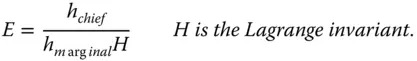

E is of course infinite at the focal point of a system. The variable is of great significance in the analysis of optical imperfections or aberrations where the distance of a component from the aperture stop is of critical importance.

These introductory chapters provide a complete description of ideal optical systems. That is to say, in the paraxial approximation, where imaging imperfections, or aberrations may be ignored, the analysis presented is substantially complete. Some very simple optical instruments are introduced at this point; their deficiencies are discussed later.