Stephen Rolt - Optical Engineering Science

Of course, for real, non-ideal imaging systems, the assumptions underlying the paraxial approximation break down. An inevitable consequence of this is the creation of imperfections or aberrations in the formation of images. A full treatment of these optical aberrations forms the subject of succeeding chapters. In the meantime, consideration of the paraxial approximation might suggest that these imperfections or aberrations would be enhanced for rays that make a large angle with respect to the optical axis. It seems sensible, therefore, to restrict rays emanating from an object to a specific, restricted range of angles. In practice, for most systems, this is done by inserting an opaque obstruction with a circular aperture. This circular aperture is centred on the optical axis and is known as an aperture stopand restricts rays emanating from an object. To further control scattered light, the aperture stop is usually blackened in some manner.

In addition to selecting rays close to the optical axis and thus reducing imperfections, aperture stops also control and define the amount of light entering an optical system. This will be explored in more detail in the chapters relating to radiometry or the study of the analysis and measurement of optical flux. Naturally, the larger the aperture, then the more light is passed through the system. Most usually, the system aperture is formed by a purpose made mechanical aperture that is distinct from the optical elements themselves. However, on occasion, the system aperture may be formed by the physical boundary of an optical component, such as a lens or a mirror. This is true, for example, for a reflecting or refracting telescope, where the boundary of the first, or primary mirror, forms the aperture stop.

This principle is illustrated in Figure 2.1which shows an object together with a corresponding aperture stop. Note that the centre of the aperture stop corresponds to the intersection of its plane with the optical axis.

The aperture stop plays an important role in image formation and the analysis of optical systems. There are a number of important definitions relating to the aperture stop and its location. Of key significance is the chief raywhich is a ray that that emanates from the object and intersects the plane of the aperture stop at its centre located at the optical axis. The angle, θ, that this ray makes with respect to the optical axis is known as the field angle. Another ray of critical importance is the marginal raythat emanates from the point where the object plane intersects the optic axis and strikes the edge of the aperture. The angle, Δ, the marginal ray makes with the axis effectively defines the size of the half angle of the cone of light emerging from a single on-axis point at the object plane and admitted by the aperture stop. The size of the aperture stop may be described either by its physical size or by the angle subtended. In the latter case, one of the most common ways of describing the aperture of an optical system is in terms of the numerical aperture(NA). The numerical aperture, is the product of the local refractive index, n, and the sine of the marginal ray angle, Δ.

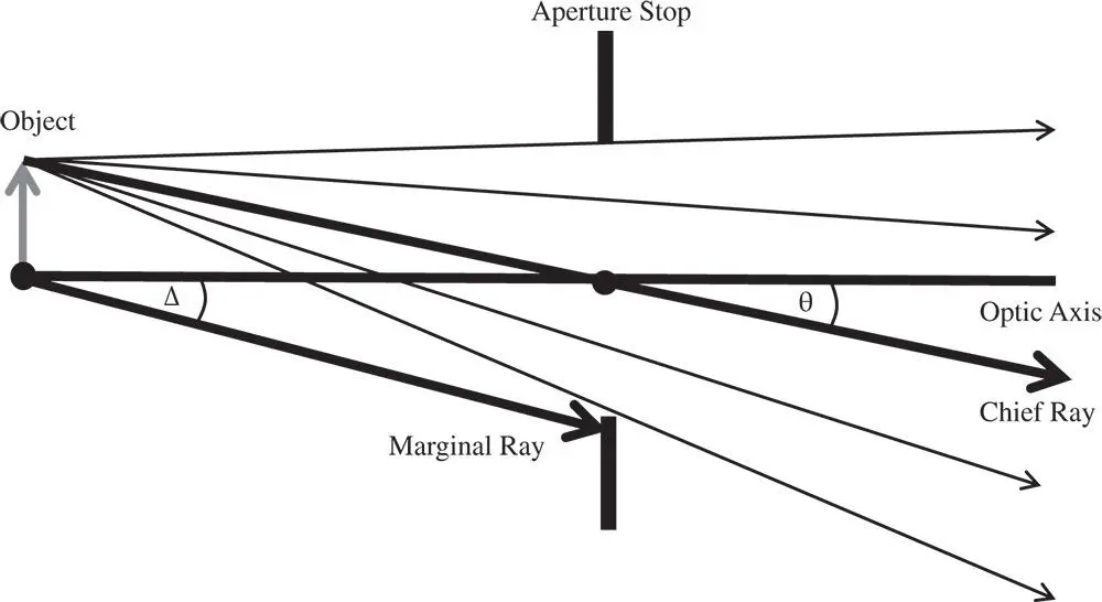
Figure 2.1 Aperture stop.

(2.1)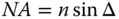

A system with a large numerical aperture, allows more light to be collected. Such a system, with a high numerical aperture is said to be ‘ fast’. This terminology has its origins in photography, where the efficient collection of light using wide apertures enabled the use of short exposure times. An alternative convention exists for describing the relative size of the aperture, namely the f-number. For a lens system, the f-number, N, is given as the ratio of the lens focal length to the aperture diameter:

(2.2)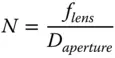

This f-number is actually written as f/N. That is to say, a lens with a focal ratio of 10 is written as f/10. The f-number has an inverse relationship to the numerical aperture and is based on the stop diameter rather than its radius. For small angles, where sinΔ = Δ, then the following relationship between the f-number and numerical aperture applies:

(2.3)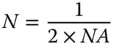

In this narrative, it is assumed that the aperture is a circular aperture, with an entire, unobstructed circular area providing access for the rays. In the majority of cases, this description is entirely accurate. However, in certain cases, this circular aperture may be partly obscured by physical or mechanical hardware supporting the optics or by holes in reflective optics. Such features are referred to as obscurations.

At this stage, it is important to emphasise the tension between fulfilment of the paraxial approximation and collection of more light. A ‘fast’ lens design naturally collects more light, but compromises the paraxial approximation and adds to the burden of complexity in lens and optical design. This inherent contradiction is explored in more detail in subsequent chapters.

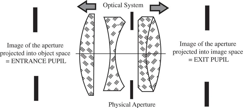
Figure 2.2 Location of entrance and exit pupils.

The physical aperture stop may not actually be located conveniently in object space as shown in Figure 2.1. On the other hand, it may be located anywhere within the sequential train of optical components that make up the optical system. An example of this is shown in Figure 2.2, a situation that is true of many camera lenses, where the physical stop is located between lenses.

In the situation described, the entrance pupilis the image of the physical aperture as projected into object space. Correspondingly, the exit pupilis the image of the physical aperture as projected into image space. The exit pupil is located in the conjugate plane to the entrance pupil and may be regarded as the image of the entrance pupil. Along with the cardinal points of a system, the location of the entrance and exit pupils are key parameters that describe an optical system. Most particularly, the numerical aperture in object space is defined by the angle of the marginal ray that intersects the edge of the entrance pupil.

Figure 2.3shows a simplified illustration of an early type of camera lens, the Cooke triplet.

By convention, image space is assumed to be on the left-hand side of the illustration. All lenses are assumed to have no tangible thickness (thin lens approximation) and the axial origin lies at the first lens. Positive axial displacement is to the right.

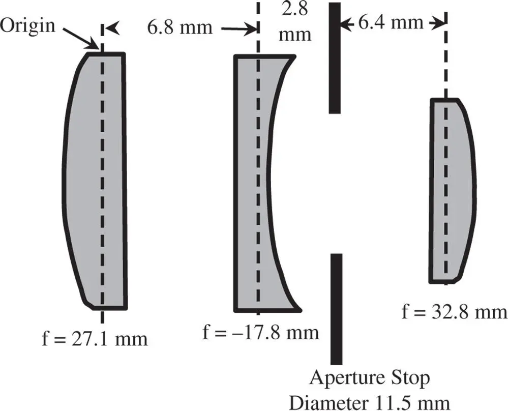
Figure 2.3 Cooke triplet.

1 Position and Size of Exit PupilIt is easiest, first of all, to calculate the position of the exit pupil, as this is the stop imaged by a single lens (the third lens) of focal length 32.8 mm. The position of the aperture stop, the object in this instance, is 6.4 mm to the left of this lens. The distance, v, of the exit pupil from the third lens is therefore given by:Thus, the exit pupil is 7.95 mm to the left of the third lens and 8.05 mm from the origin. The magnification is given by (minus) the ratio of image and object distances and so it is easy to calculate the size of the exit pupil: