Stephen Rolt - Optical Engineering Science

(1.26)

Note the order of the multiplication; this is important. M 1represents the first optical element seen by rays incident upon the system and the multiplication procedure then works through elements 2–6 successively. For purposes of illustration, each lens has been treated as being represented by a single matrix element. In practice, it is likely that the lens would be reduced to its basic building blocks, namely the two curved surfaces plus the propagation (thickness) between the two surfaces.We also must not forget the propagation through the air between the lens elements.

Representation of the key optical surfaces can be determined by casting Eqs. (1.18)– (1.22)in matrix format.

(1.27a)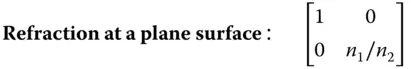

(1.27b)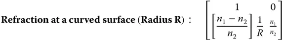

(1.27c)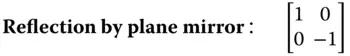

(1.27d)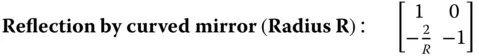

(1.27e)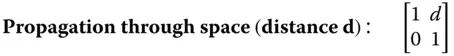

(1.27f)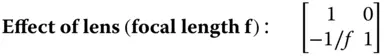

n 1and n 2represent the refractive index of first and second media respectively.

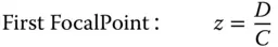
It is very straightforward to calculate the Cardinal Points of a system from the system matrix:

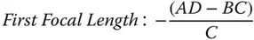
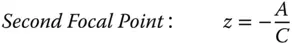
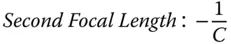
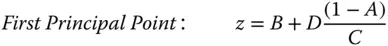
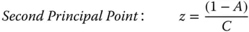
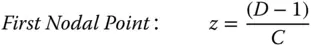
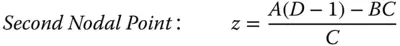
The matrix above represents the system matrix after propagating through all optical elements as shown in Figure 1.17. However, the convention adopted here is that an additional transformation is added after the final surface. This additional transformation is free space propagation to the original starting point. It must be emphasised that, this is merely a convention, and that the final step traces a dummy rayas opposed to a real ray. That is to say, in reality, the light does not propagate backwards to this point. In fact, this step is a virtual back-projection of the real ray which preserves the original ray geometry. The logic of this, as will be seen, is that in any subsequent analysis, the location of all cardinal points is referenced with respect to a common starting point. If this step were dispensed with, then the three first Cardinal Points would be referenced to the start point and the three second Cardinal Points to the end point. With this in mind, the Cardinal Points, as referenced to the common start point are set out below; the reader might wish to confirm this.

The determinantof the matrix, ( AD−BC), is a key parameter. The ratio of the two focal lengths of the system is simply given by the determinant. That is to say the ratio of the two focal lengths is given by:

(1.28)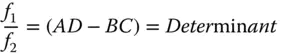

Inspecting all matrix expressions in Eqs. (1.27a– 1.27f), the determinant of the matrix is simply n 1/n 2, the ratio of the indices in the two media, for all possible scenarios. Since the determinant of a matrix product is simply the product of the individual determinants, then the determinant of the overall system matrix is simply the ratio of the refractive indices in image and object space. Thus:

(1.29)

This relationship was anticipated in the more generalised discussion in 1.3.9. Looking at the relationships for the principal and nodal points, it is clear when the determinant of the system matrix is unity, i.e. object and image space indices are the same, then the principal and nodal points are co-located.

In addition to the principal and nodal points, anti-principal pointsand anti-nodal pointsare sometimes (rarely) specified. Anti-principal points are conjugate points where the magnification is −1. Similarly, anti-nodal points are conjugate points where the angular magnification is −1.

We can now use the foregoing analysis to see how matrix ray tracing might be used in practice. Here we focus on a number of useful practical examples.

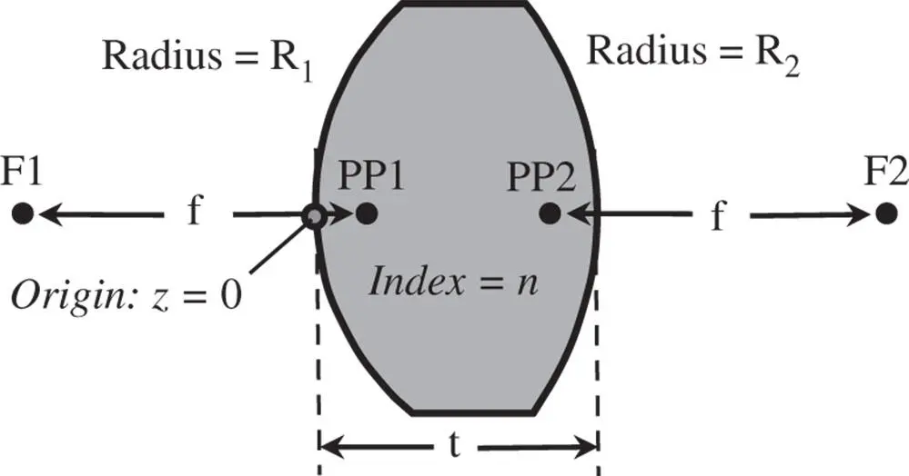
Figure 1.19 Thick lens.

The matrix for the system is simply as below – note the order:

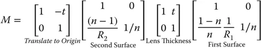
We have two translations. The first translation represents the thickness of the lens and the second translation, by convention, traces the refracted rays back to the origin in z . This is so that, in interpreting the formulae for Cardinal points, we can be sure that they are all referenced to a common origin, located as in Figure 1.19. Positive axial displacement ( z ) is to the right and a positive radius, R , is where the centre of curvature lies to the right of the vertex. The final matrix is as below: