Stephen Rolt - Optical Engineering Science

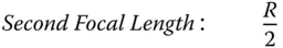
As with the curved refractive surface, a curved mirror is image forming. It is therefore possible to set out the Cardinal Points, as before: Cardinal points for a spherical mirror

Both Principal Points: At vertex
Both Nodal Points: At centre of sphere

The focal length of a curved mirror is half the base radius, with both focal points co-located. In fact, the two focal lengths are of opposite sign. Again, this fits in with the notion that reflective surfaces act as media with a refractive index of −1. Both nodal points are co-located at the centre of curvature and the principal points are also co-located at the surface vertex.

Earlier, in order to make our lens and mirror calculations simple and tractable, we introduced the following approximation:

That is to say, all rays make a sufficiently small angle to the optical axis to make the above approximation acceptable in practice. When this approximation is applied more generally to an entire optical system, it is referred to as the paraxial approximation(i.e. ‘almost axial’ ). If the same consideration is applied to ray heights as well as angles, the paraxial approximations lead to a series of equations describing the transformation of ray heights and angles that are linear in both ray height and angle. This first order theory is generally referred to as Gaussian optics, named after Carl Friedrich Gauss.

If we now assume that all rays are confined to a single plane containing the optical axis, then we can describe all rays by two parameters: θ – the angle the ray make to the optical axis and h – the height above the optical axis. If, after transformation by an optical surface, these parameters change to θ′ and h′, it is possible to write down a series of linear equations describing all transformations. These are set out in Eqs. 1.18– 1.21:

(1.18)

(1.19)

(1.20)

(1.21)

Even the most complex optical system may be described as a combination of all the above elements. At first sight, therefore, it would seem that this provides a complete description of the first order behaviour of an optical system. However, there is one important, but seemingly trivial, aspect that is not considered here. This is the case of ray propagation through space. The equations are, of course simple and obvious, but we include them for completeness.

(1.22)

Equation (1.8)introduced the Helmholtz equation, a necessary condition for perfect image formation for an ideal system. It is clear that Gaussian optics represents a mere approximation to the ideal of the Helmholtz equation. The contradiction between the two suggests that there may be imperfections in the ideal treatment of Gaussian optics. This will be considered later when we will look at optical imperfections or aberrations. In the meantime, we will consider a very powerful realisation of Gaussian optics that takes the basic linear equations previously set out and expresses them in terms of matrix algebra. This is the so-called Matrix Ray Tracing technique.

In Section 1.4we looked at the behaviour of some very simple components, mirrors and lenses, deriving the locations of the Cardinal Points. As discussed previously, the Cardinal Points provide a complete description of the first order properties of an optical system, no matter how complex.

The question then is how do we calculate the properties of a more complex optical system, such as the camera lens depicted in Figure 1.17? It is not immediately obvious where the Cardinal points lie or what the focal length is. However, we can combine the generalised description of an optical system with the treatment of Gaussian optics to produce a model that describes the entire system as a black box acting on rays with a simple linear transformation. The black box may be visualised as below in Figure 1.18.

Following the basic premise of Gaussian optics, we can relate the input and output rays using a set of linear equations:

(1.23)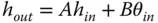

(1.24)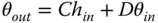

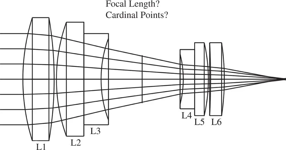
Figure 1.17 Complex optical system.

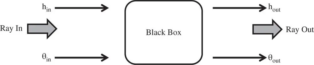
Figure 1.18 Modelling of complex systems.

Equations (1.23)and (1.24)may be combined in a matrix representation:

(1.25)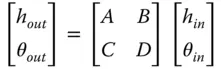

Equation (1.25)sets out the Matrix Ray Tracingconvention used in this book. The reader should be aware that other conventions are used, but this is the most widely used. Equation (1.25)can be used to describe the overall system matrix or that of individual components. The question is how to build up a complex system from a large number of optical elements. The camera lens shown in Figure 1.17has six lenses and we might represent each lens as a single matrix, i.e. M 1 , M 2 ,…..,M 6. Each matrix describes the relationship between rays incident upon the lens and those leaving. The impact of successive optical elements is determined by successive matrix multiplication. So the system matrix for the lens as a whole is given by the matrix product of all elements: