Stephen Rolt - Optical Engineering Science

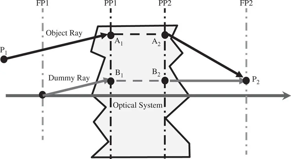
Figure 1.9 Tracing of arbitrary ray.

The angular magnificationof an optical system is the ratio of the angle (with respect to the optical axis) of a ray in image space and that of its conjugate in object space. There exists a pair of conjugate points lying on the optical axis where, for all possible rays, the angular magnification is unity. These are the nodal points. The first nodal pointis located in object space and the second nodal pointis located in image space. This is set out in Figure 1.10, where for a general conjugate pair, the angular magnification, α, is equal to θ 2/θ 1. For the nodal points, θ 2= θ 1; that is to say, the angular magnification is unity. Where the two focal lengths are identical, or the object and image spaces are within media of the same refractive index, the nodal points are co-located with the principal points.

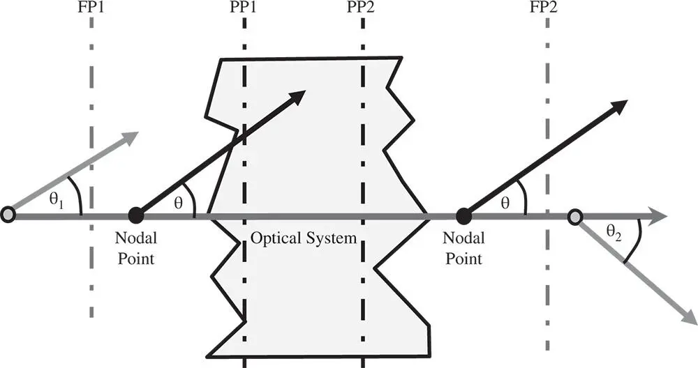
Figure 1.10 Angular magnification and nodal points.

This brief description has provided a complete definition of an ideal optical system. No matter how complex (or simple) the optical system, this analysis defines the complete end-to-end functionality of an ideal system. On this basis, an optical designer will specify the six cardinal pointsof a system to describe the ideal behaviour of a design. These six cardinal points are:

First Focal Point

Second Focal Point

First Principal Point

Second Principal Point

First Nodal Point

Second Nodal Point

The principal and nodal points are co-located if the two system focal lengths are identical.

The location of the cardinal points has given us a complete description of a generalised optical system. Given that the function of an optical system might be to produce an image of an object located at a specific point, we might want to know the location of that image. Figure 1.11shows the relationship between a generalised object and image.

Referring to Figure 1.11and by using similar triangles it is possible to derive two separate relations for the magnification h 2/ h 1:

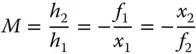
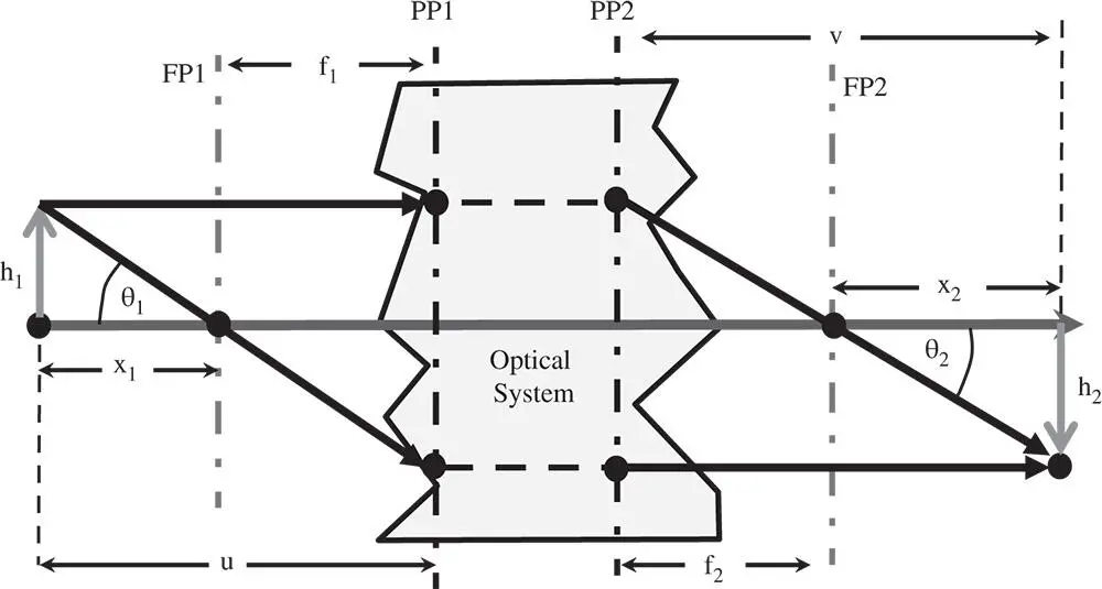
Figure 1.11 Generalised object and image.

And:

(1.6)

The above equation is Newton's Equationand may be re-cast into a more familiar form using the definitions of object and image distances, u and v, as previously set out.

(1.7)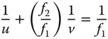

If f 1= f 2= f , we are left with the more familiar lens equation. However, Eq. (1.7)is generally applicable to all optical systems. Most importantly, Eq. (1.7)will give the locations of the object and image in systems of arbitrary complexity. Many readers might have encountered Eq. (1.7)in the context of a simple lens where object and image distances are obvious and easy to determine. For a more complex system, one has to know the location of the principal planes as well in order to determine the object and image distances.

Thus far, we have presented a description of an idealised optical system. Is there a simple condition that needs to be fulfilled in order to generate such an ideal image? It is easy to see from Figure 1.11that the following relations apply:

Therefore:

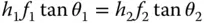
As we will be able to show later, the ratio f 2/ f 1is equal to the ratio of the refractive indices, n 2/ n 1, in the two media (object and image space). Therefore it is possible to cast the above equation in its more usual form, the Helmholtz equation:

(1.8)

One important consequence of the Helmholtz equation is that there is a clear, inextricable linkage between transverse and angular magnification. Angular magnification is inversely proportional to transverse magnification. For small θ, tan θ and θ are approximately equal. So in the small signal approximation, the angular magnification, α is given by:

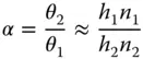
Hence:

(1.9)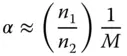

We have, thus far, introduced two different types of optical magnification – transverse and angular. There is a third type of magnification that we need to consider, longitudinal magnification. Longitudinal magnitude, L , is defined as the shift in the axial image position for a unit shift in the object position, i.e.:

(1.10)

From Newton's Eq. (1.6):

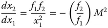
And:

(1.11)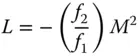

Thus, the longitudinal magnification is proportional to the square of the transverse magnification.

The analysis presented thus far is entirely independent of the optical components that might populate the idealised optical system. In this section we will begin to consider, from the perspective of ray optics, the behaviour of real elements that make up this generalised system. At a basic level, only a few behaviours need to be considered in order to understand the propagation of rays through a real optical system. These are: