Stephen Rolt - Optical Engineering Science

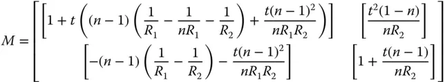
As both object and image space are in the same media, there is a common focal length, f , i.e. f 1= f 2= f . All relevant parameters are calculated from the above matrix using the formulae tabulated in Section 1.6.2.

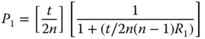
The focal length, f , is given by:

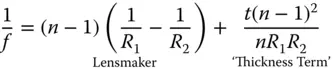
The formula above is similar to the simple, ‘Lensmaker’ formula for a thin lens. In addition there is another term, linear in thickness, t , which accounts for the lens thickness.

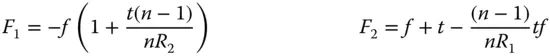
The focal positions are as follows:

The principal points are as follows:

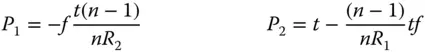
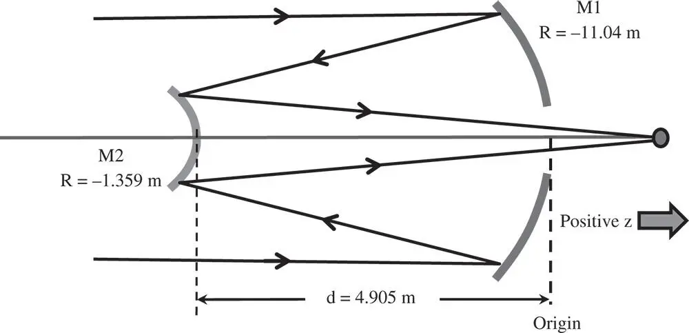
Figure 1.20 Hubble space telescope schematic.

Of course, since the refractive indices of the object and image spaces are identical, the nodal points are located in the same place as the principal points. If we take the example of a biconvex lens where R 2= −R 1, then:

So, for a biconvex lens with a refractive index of 1.5, then the principal points lie about one third of the thickness from their respective vertices.

The telescope part of the Hubble Space Telescope instrument is made up of two mirrors, a primary and a secondary. Characteristics of the telescope are shown in Figure 1.20. Data is courtesy of the National Aeronautics and Space Administration .

There are four matrix elements to consider here. First, there is a mirror with a radius of −11.04 m (note sign), followed by a translation of −4.905 m (again note sign). The third matrix element is a mirror (M2) of radius − 1.359 m. Finally, we translate by +4.905 m, so that both the input and output co-ordinates are referenced with respect to the same origin. The matrices are as below:

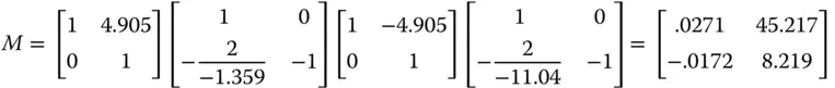
The focal positions are:

The principal points are at:

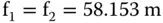
Since object and image space are in the same media, then the two focal lengths are the same. In addition, the nodal and principal points are co-located. However, when dealing with mirrors, one must be a little cautious. Each reflection is equivalent to a medium with a refractive index of −1, so that the matrix of a reflective surface will always have a determinant of −1. Therefore, any system having an even numberof reflective surfaces, as in this example, then its matrix will have a determinant of 1. As such, the two focal lengths will be the same and principal and nodal points co-located. However, where there are an odd numberof reflective surfaces, assuming object and image spaces are surrounded by the same media, then f 2= − f 1. In this instance, principal and nodal points are separated by twice the focal length.

Although, in terms of overall length, the telescope is compact, ∼5 m primary–secondary separation, the focal length, at 58 m, is long. The focal length of the instrument is fundamental in determining the ‘plate scale’ the separation of imaged objects (stars, galaxies) at the (second) focal plane as a function of their angularseparation. As such, a long focal length, of the order of 60 m, may have been a requirementat the outset. At the same time, for practical reasons, a compact design may also have been desired. One may begin to glance, therefore, at the significance, at the very outset of these very basic calculations in the design of complex optical instruments.

For the examples previously set out, matrix multiplication is a quick and convenient method for calculating the first order parameters of an optical system. Nonetheless, it must be recognised that as systems become more complex, with more optical surfaces, these calculations can become quite tedious. However, these matrix calculations are easy to embed with spreadsheet tools enabling the automatic computation of all cardinal points. By way of example, the previous calculation is set out and automated using a simple spreadsheet tool.

In the exercises that follow, the reader may choose to use this method to simplify calculations.

1 Born, M. and Wolf, E. (1999). Principles of Optics, 7e. Cambridge: Cambridge University Press. ISBN: 0-521-642221.

2 Haija, A.I., Numan, M.Z., and Freeman, W.L. (2018). Concise Optics: Concepts, Examples and Problems. Boca Raton: CRC Press. ISBN: 978-1-1381-0702-1.

3 Hecht, E. (2017). Optics, 5e. Harlow: Pearson Education. ISBN: 978-0-1339-7722-6.

4 Keating, M.P. (1988). Geometric, Physical, and Visual Optics. Boston: Butterworths. ISBN: 978-0-7506-7262-7.

5 Kidger, M.J. (2001). Fundamental Optical Design. Bellingham: SPIE. ISBN: 0-81943915-0.

6 Kloos, G. (2007). Matrix Methods for Optical Layout. Bellingham: SPIE. ISBN: 978-0-8194-6780-5.

7 Longhurst, R.S. (1973). Geometrical and Physical Optics, 3e. London: Longmans. ISBN: 0-582-44099-8.

8 Riedl, M.J. (2009). Optical Design: Applying the Fundamentals. Bellingham: SPIE. ISBN: 978-0-8194-7799-6.

9 Saleh, B.E.A. and Teich, M.C. (2007). Fundamentals of Photonics, 2e. New York: Wiley. ISBN: 978-0-471-35832-9.

10 Smith, F.G. and Thompson, J.H. (1989). Optics, 2e. New York: Wiley. ISBN: 0-471-91538-1.

11 Smith, W.J. (2007). Modern Optical Engineering. Bellingham: SPIE. ISBN: 978-0-8194-7096-6.

12 Walker, B.H. (2009). Optical Engineering Fundamentals, 2e. Bellingham: SPIE. ISBN: 978-0-8194-7540-4.

In the previous chapter, we were introduced to sequential geometric optics. The simple analysis presented there is contingent upon the paraxial approximation. It is assumed that all rays in their sequential progress through the optical system always subtend a negligibly small angle with respect to the optical axis. In this scenario, the effect of all optical elements may be described in terms of a simple set of linear (in ray height and angle) equations leading to perfect image formation. This analysis, as previously outlined, is referred to as Gaussian optics.