Stephen Rolt - Optical Engineering Science

2 Cardinal Points of the LensThe distance between the first and second lenses is 6.8 mm and between the second and third lenses is 9.2 mm. By convention, we retrace dummy rays −16 mm back to the origin at the first lens, so that all matrix ray tracing formulae are referred to a common origin. The matrix for the system is given below:To calculate the position of the exit pupil we need to know the focal length of the system and the positions of the two focal points. Following the matrix relations set out in Chapter 1, we can calculate the following:Focal length: 52.3 mmLocation of First Focal Point: −41.2 mmLocation of Second Focal Point: 57.7 mmAll distances are referenced to the axial origin at the first lens. There is, of course, a single effective focal length as both object and image spaces are considered to lie within media of the same refractive index.

3 Position and Size of the Entrance PupilThe imaged pupil or exit pupil lies in image space, 8.05 mm from the origin. This is 49.65 mm to the left of the second focal point. In applying Newton's formula, the second focal distance, x2 is then equal to −49.65. We can now calculate the first focal distance to determine the position of the entrance pupil.The object or entrance pupil therefore lies 55.1 mm to the right of the first focal point and 13.9 mm (−41.2 + 55.1) to the right of the first lens.The location of the entrance pupil expressed as an object distance is 52.3 − 55.1 or −2.8 mm. Similarly the location of the exit pupil expressed as an image distance is equal to −49.65 + 52.3 or +2.65 mm. The magnification (image/object) is, in this instance equal to 2.65/2.8 or 0.946. Therefore we have:The diameter of the entrance pupil is, therefore, 15.1 mmSo, in summary we have:

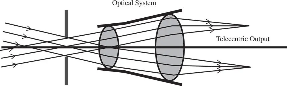
Figure 2.4 Optical system with a telecentric output.

In the previous example, both entrance and exit pupils were located at finite conjugates. However, a system is said to be telecentricif the exit pupil (or entrance pupil) is located at infinity. In the case of a telecentric output, this will occur where the entrance pupil is located at the first focal point. In this instance, all chief rays will, in image space, be parallel. This is shown in Figure 2.4which illustrates a telecentric output for two different field positions.

A telecentric output, as represented in Figure 2.4is characterised by a number of converging ray bundles, each emanating from a specific field location, whose central or chief rays are parallel. There are a number of instances where optical systems are specifically designed to be telecentric. Telecentric lenses, for instance, have application in machine vision and metrology where non-telecentric output can lead to measurement errors for varying (object) axial positions.

The aperture stop is the principal means for controlling the passage of rays through an optical system. Ideally, this would be the only component that controls the admission of light to the optical system. In practice, other optical surfaces located away from the aperture stop may also have an impact on the admission of light into the system. This is because these optical components, for reasons of economy and other optical design factors, have a finite aperture. As a consequence, some rays, particularly those for larger field angles, may miss the lens or component aperture altogether. So, in this case, for field positions furthest from the optical axis, some of the rays will be clipped. This process is known as vignetting. This is shown in Figure 2.5.

Vignetting tends to darken the image for objects further away from the optical axis. As such, it is an undesirable effect. At the same time, it can be used to control optical imperfections or aberrations by deliberately removing more marginal rays.

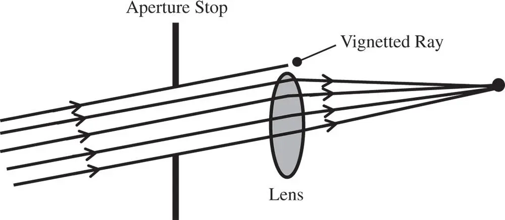
Figure 2.5 Vignetting.

In addition to the aperture stop, an optical system might also contain a field stop. This is an aperture located in a plane that is conjugate with the image plane. Its first purpose is to provide a crisp (often circular) boundary to the viewable image. Secondly, it excludes light from object locations lying outside the area of interest. In so doing, the field stop reduces the level of unwanted light that might otherwise be scattered into the image plane and so reduce image contrast. For the same reason, other, intermediate stops may be introduced into an optical design in order to further reduce the level of scattered light.

The analysis pursued hitherto has considered the propagation of rays in a single plane. From an analytical perspective, for ray tracing in an ideal system and determining the cardinal points of that system, this is a perfectly acceptable approach. However, in reality, rays are not necessarily confined to the plane containing the object and the optical axis. With the selection of rays delineated by a two-dimensional, circularaperture, we must expect some rays to be out of this plane. A group of co-planar rays, emanating from a single object point and bounded by the entrance pupil is referred to as a ray fan. A ray fan that lies in the plane defined by the object and optical axis is known as the tangential ray fan. The sagittal ray fan emanates from the same object point and lies in a plane that is perpendicular to that of the tangential ray fan. This is illustrated in Figure 2.6.

The tangential ray fan is also referred to as the meridional ray fan; the two terms are equivalent. In general any ray that is not in the tangential plane, i.e. not a tangential ray, is referred to as a skew ray. A skew ray will never cross the optic axis.

The introduction of two distinct sets of ray fans, tangential and sagittal, together with the inclusion of skew rays confirms that sequential ray propagation in an axial geometry is essentially a two-dimensional problem. Hitherto, all discussion and, in particular, the matrix analysis, has been presented in a strictly one-dimensional form. However, the strict description of a ray in two dimensions requires the definition of four parameters, two spatial and two angular. In this more complete description, a ray vector would be written as:

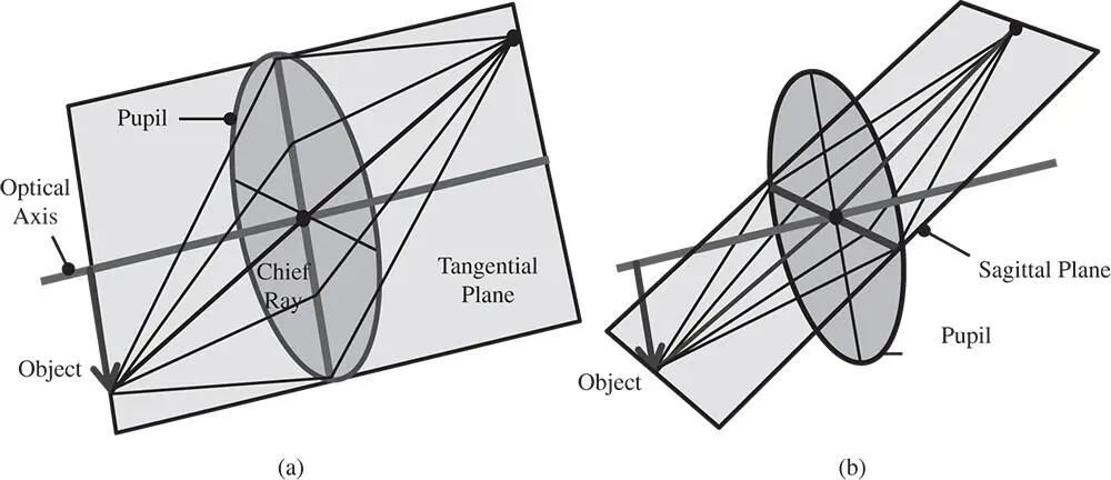
Figure 2.6 (a) Tangential ray fan; (b) Sagittal ray fan.

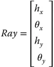
hx is the x component of the distance of the ray from the optical axis

θx is the x component of the angle of the ray to the optical axis

hy is the y component of the distance of the ray from the optical axis

θy is the y component of the angle of the ray to the optical axis