Joel P. Dunsmore - Handbook of Microwave Component Measurements

From inspection, one can recognize that the waves a 2A= b 1Band b 2A= a 1Bso that the concatenation becomes this simple result

(2.22)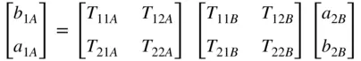

Or

(2.23)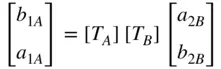

Using this definition of T‐parameters, the following conversions can be defined

(2.24)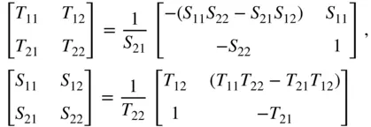

Note that in this conversion, S21 always appears in the denominator. This can cause numerical difficulties in devices with transmission zeros and can sometimes cause de‐embedding functions to fail. More robust de‐embedding algorithms check for this condition and modify the method of concatenation in such a case.

Other definitions of T‐parameter type relationships have been described, which exchange the position variables a 1and b 1on the dependent variable side and exchange the position of a 2and b 2on the independent variable side (Mavaddat 1996). This version has similar properties, but care must be taken not to confuse the two methods as, of course, the resulting T‐parameters are different. Another definition, which might seem more intuitive, would set the input terms a 1and b 1as the independent variable. Unfortunately, this has the undesirable effect of setting S12 in the denominator of the transformation parameter and thus gives difficulties when applied to unilateral gain devices such as amplifiers.

One common desire in evaluating the performance of a component is to model that component as an impedance comprised of a resistive element with a single series or shunt reactive element, as demonstrated in Section 2.4.1.1. This desire was furthered by some built‐in transformation functions on VNAs, first introduced with the HP8753A but common now on many models. The goal was to model a device in such a way that the S‐parameters mapped to a single resistive and reactive element in the so‐called Z‐transform case (not to be confused with the discrete time z‐transform) or a single conductance and susceptance in the Y‐transform case. These are quite simple models and represented in Figure 2.40.

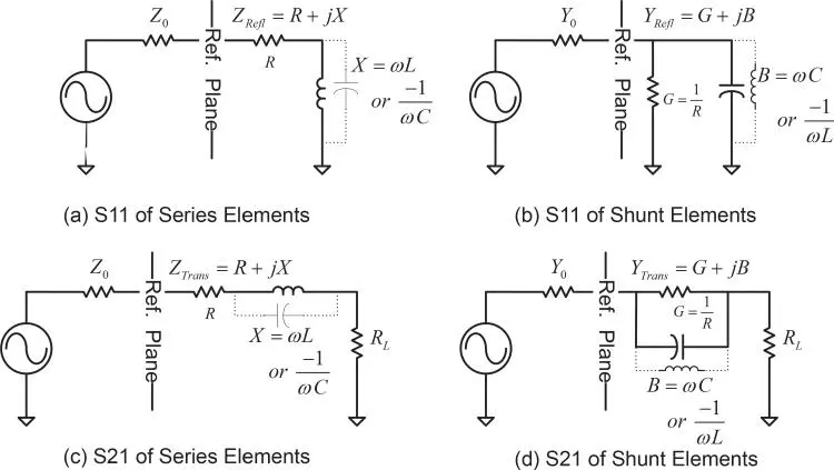
Figure 2.40 Y and Z conversion circuits.

Reflection conversions are computed from the S11 trace and are essentially the same values as presented by impedance or admittance readouts of the Smith chart markers. Thus, Z‐reflection conversion would be used with the circuit description from Figure 2.40a and display the impedance in the real part of the result and the reactance in the imaginary part of the result. Y‐reflection would be used with the circuit of Figure 2.40b and display the conductance in the real part and the susceptance in the imaginary part of the result. The computations for these conversions are

(2.25)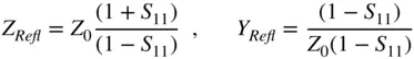

Typically, these conversions would be used on one‐port devices and measurements. If it is used on a 2‐port device, one must remember that the load impedance will affect the measured value of the Z‐ or Y‐reflected conversion.

These reflection conversions are already well known as the models represented by the Smith chart, but a similar conversion can be performed for a simple transmission measurement. In this case, the circuits of Figure 2.40c and Figure 2.40d are the reference circuits for these conversions. They are useful when analyzing the series element models, such as coupling capacitors, and the models for series resistors and inductors. The underlying computation for the transmission conversions is

(2.26)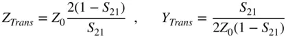

The Z‐transmission conversion would be well suited to view the series resistance of a coupling capacitor. The Y‐transmission would show the resistive value of a series‐mounted surface‐mount technology (SMT) resistor with a shunt capacitance as a constant conductance with a reactance increasing as 2 πf , forming a straight reactance line.

These conversions are often confused with conversion to Y‐ or Z‐parameters, but they are not, in general, related. These provide simple modeling functions based on a single S‐parameter, whereas the Y‐, Z‐, and related parameters provide a matrix result and require knowledge of all four S‐parameters as well as the reference impedance. These other matrix parameters are described in the next section.

Even though a VNA measures S‐parameters as its fundamental information, many other figures of merit may be computed directly from these measurements, through the use of transformations, found in several references (Hong and Lancaster 2001; Keysight Technologies n.d.-a). Most of these common parameters relate the voltage and current at the ports, rather than the a and b waves. Many of these transformations arise out of different definitions of terminal conditions as applied to Figure 1.2. These definitions arise out of DC or low‐frequency measurements, where it is an easy matter to short a terminal, meaning Z L= 0, or open a terminal, meaning Z L→ ∞. An often confusing point is that it is not necessary that the terminals actually be opened or shorted, but most commonly the parameter is described in those terms. Just as it is most common to terminate the a 2‐port network in Z 0to define S21, making a 2= 0, it is not necessary to do so, and S21 can be determined with any terminal impedance as long as sufficient changes in a1 and a2 are made to solve Eq. (1.17), as shown in Eq. (1.21). Since the voltage and current relationships on the terminals of a DUT are easily determined from the S‐parameters, many other linear parameters can be determined as well. Unless otherwise noted, these transformations apply to the simple case where the S‐parameters are defined with a single, real‐valued reference impedance.

Z‐parameters are one of the more commonly defined parameters and often the first characterization parameter introduced in engineering courses on electrical circuit fundamentals.

The Z‐parameters are defined in terms of voltages and currents on the terminals as

(2.27)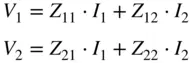

where the V's and I's are defined in Figure 1.2. If we apply the condition of driving a voltage source into the first input terminal and opening the first output terminal, which forces I 2to zero, and measure the input and output voltages, we can determine two of the parameters; similarly, the other two parameters are determined by driving the output terminal and opening the input terminal. Mathematically this can be stated as