Joel P. Dunsmore - Handbook of Microwave Component Measurements

A second cause of trace noise in a measurement is called high‐level trace noise. At high signal levels, the noise from the source signal, typically due to the phase noise of the source, can rise above the VNA noise floor and dominate the trace noise in the measurement. Further, if the source in the VNA has substantial internal amplification, the broadband noise floor from the source can dominate the phase noise far from the carrier. In this region, the trace noise stays approximately the same as the S‐parameter signal increases. Consider the trace noise on the skirt of a filter: when the signal through the filter is sufficiently high, the trace noise on the measurement decreases as the signal level rises above the noise floor, until the source phase noise or pedestal noise, as it is sometimes called, becomes dominant. Above this level the trace noise stays constant as a dBc level even as the S‐parameter loss diminishes. The problem of high‐level trace noise is more commonly found on older VNAs where phase noise was typically worse than that of stand‐alone signal sources due to the difficulty of integrating sources internally. The problem is also seen on more modern VNA systems at mm‐wave frequency, where multipliers are used to increase the source frequency. With each 2x multiplication of frequency, the phase noise increases by 6 dB. These problems are typically seen only at high power levels because the use of attenuators for power‐level control reduces the source signal and the phase noise in the same manner.

Figure 2.33shows the phase noise of a VNA source as it is increased to where the phase noise is higher than the noise floor. The memory trace, shown in light gray, is for a power level of −10 dBm. At this level phase noise is below the receiver noise floor. The dark trace shows the phase noise when the source power is increased to +10 dBm. Here the phase noise is about 15 dB above the noise floor and will limit the high‐level trace noise. This data was measured with a 10 kHz resolution bandwidth (RBW), so the actual maximum phase noise is about −110 dBc Hz −1at offsets below about 50 kHz.

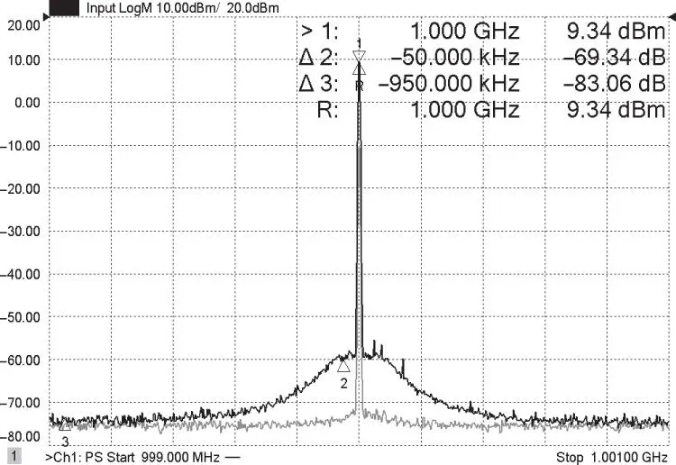
Figure 2.33 VNA source signal where phase noise rises above noise floor.

Figure 2.34shows a plot of trace noise as a function of received power. In this normalized response, the trace noise limit is apparent in the high‐level region starting at about −10 dBm, where the trace noise no longer decreases directly as a function of increased signal level, indicated on the figure as the “Hi‐Level Trace Noise” region.

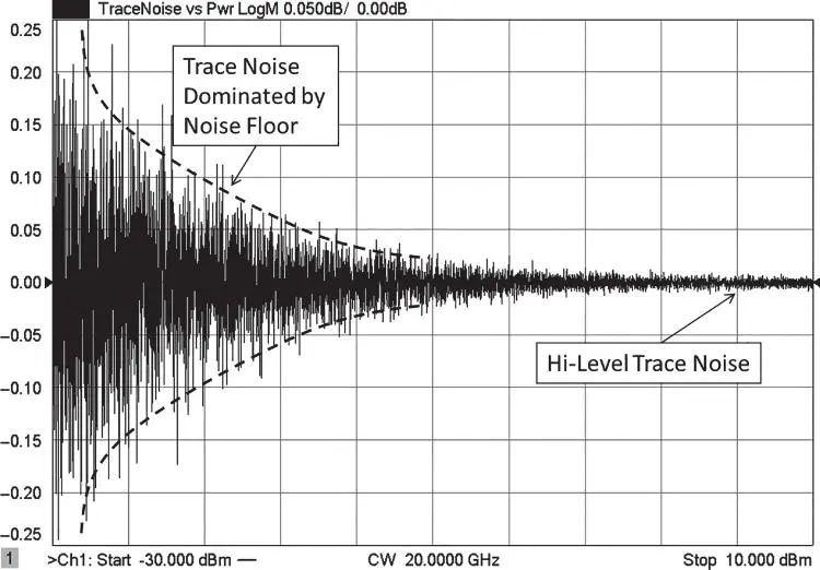
Figure 2.34 Example of trace noise decreasing with increased signal level, until high level noise limit is reached.

Often, the performance of external components used to connect from the VNA to the DUT presents the largest contribution of errors to the measurement. These errors can come in a variety of configurations, and each has its own peculiarities that can affect measurements in different ways. The most common causes of external errors are cables and connectors.

Cables, connectors, and adapters are ubiquitous when using VNAs to measure most devices. The quality and particularly the stability of the cable and connector can dramatically affect the quality of the measurement.

The first‐order effect of cables is added loss and mismatch in a measurement. For short cables, the loss is not significant, but the mismatch can add directly to the source‐match and directivity of the VNA to degrade performance. With error correction, the effect of mismatch can be substantially reduced (to the level of the calibration standards quality) if it is stable, but cable instability limits the repeatability of the cable mismatch and often is the dominant error in a return‐loss measurement.

For transmission measurements, the effects of mismatch do directly affect calibration, though it is reduced to a small level by the quality of the calibration standards. Often, the major instability in a cable is the phase response versus frequency. Even if the amplitude of the cable is stable, if the phase response changes, the VNA error correction will become corrupted because of phase shift of the cable mismatch error. Methods for determining the quality of cable and the effects of flexure will be described in Chapter 9.

S‐parameter measurements provide substantial information about the qualities of a DUT. In many cases, the transformation and formatting of these parameters is necessary to more readily understand the intrinsic attributes of the DUT. Some of these transformations are graphical in nature, such as plotting on a Smith chart; some are formatting such a group delay and SWR; and some are functional transformation such as time‐domain transforms. Some of the more important transformations are discussed next, with emphasis on some particularly interesting results.

The Smith chart is a visualization tool that every RF engineer should strive to master. It provides a compact form for describing the match characteristics of a DUT, as well as being a useful tool for moving the match point of a device to a more desired value. Invented by Philip Smith (1944), it maps the normalized complex value of a termination impedance onto a circular‐based chart, from which the impedance effects of adding lengths of transmission line onto the termination impedance are easily computed. The original intention for the use of a Smith chart was for the computing of impedances presented to a generator as lengths of transmission line were added to a load and was intended particularly for the use of telephone line impedance matching. Adding a length of transmission lines changes the apparent termination impedance, Z T, according to

(2.14)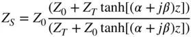

where α and β are the real and imaginary propagation constants, and z is the distance from the load. This computation was tedious, in part because the argument of the hyperbolic tangent is complex, so a nomographic approach was desirable. A Smith chart solves by this mapping impedance to reflection coefficient (Γ), and plotting the return loss on a polar plot, as

(2.15)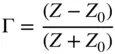

The genius of the Smith chart is recognizing that rotating an impedance value through a length of transmission line is the same as rotating the phase of the reflection coefficient value on the chart. The Smith chart maps the impedance onto the polar reflection coefficient plot, but with the graticule lines marked with circles of constant resistance and circles of constant reactance. As such, any return loss value can be plotted, and the equivalent resistance and reactance can be determined immediately. To see the effect of adding some Z 0transmission line, the impedance is simply rotated on the polar plot by the phase shift of the transmission line. If the line is lossy, the return loss is modified by the line loss (two times the one‐way loss of the line), and from this new position, the resistance and the reactance are directly read.