Claude Cohen-Tannoudji - Quantum Mechanics, Volume 3

To obtain the matrix elements of in the representation {| r, ν )}, we use (85)after replacing the | θ 〉 by the | φ 〉 (we showed in § 3 that this was possible). We now multiply both sides by and , and sum over the subscripts k and l ; we recognize in both sides the closure relations:

(92)

This leads to:

(93)

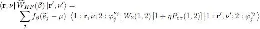
As in § C-5 of Chapter XV, we get the sum of a direct term (the term 1 in the central bracket) and an exchange term (the term in η P ex). This expression contains the same matrix element as relation (87)of Complement E xv, the only difference being the presence of a coefficient in each term of the sum (plus the fact that the summation index goes to infinity).

(i) For the direct term, as we did in that complement, we insert a closure relation on the particle 2 position:

(94)

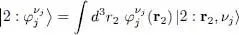
Since the interaction operator is diagonal in the position representation, the part of the matrix element of (93)that does not contain the exchange operator becomes:

(95)

The direct term of (93)is then written:

(96)

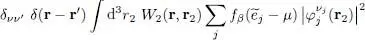
which is equivalent to relation (91)of Complement E XV.

(ii) The exchange term is obtained by permutation of the two particles in the ket appearing on the right-hand side of (93); the diagonal character of W 2(1,2) in the position representation leads to the expression:

(97)

For the first scalar product to be non-zero, the subscript j must be such that νj = ν ; in the same way, for the second product to be non-zero, we must have νj = ν′ . For both conditions to be satisfied, we must impose ν = ν ′, and the exchange term (93)is equal to:

(98)

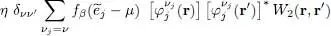
where the summation is on all the values of j such that νj = ν : this term only exists if the two interacting particles are totally indistinguishable, which requires that they be in the same spin state (see the discussion in Complement E XV).

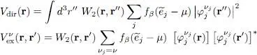
We now define the direct and exchange potentials by:

(99)

The equalities (87)then lead to the Hartree-Fock equations in the position representation:

(100)

The general discussion of § 3-b can be applied here without any changes. These equations are both nonlinear and self-consistent, as the direct and exchange potentials are themselves functions of the solutions of the eigenvalue equations (100). This situation is reminiscent of the zero-temperature case, and we can, once again, look for solutions using iterative methods. The number of equations to be solved, however, is infinite and no longer equal to the finite number N , as already pointed out in § 3-c. The set of solutions must span the entire individual state space. Along the same line, in the definitions (99)of the direct and exchange potentials, the summations over j are not limited to N states, but go to infinity. However, even though the number of these wave functions is in principle infinite, it is limited in practice (for numerical calculations) to a high but finite number. As for the initial conditions to start the iteration process, one can choose for example the states and energies of a free fermion gas, but any other conjecture is equally possible.

There are many applications of the previous calculations, and more generally of the mean field theory. We give a few examples in the next complement, which are far from showing the richness of the possible application range. The main physical idea is to reduce, whenever possible, the calculation of the various physical quantities to a problem similar to that of an ideal gas, where the particles have independent dynamics. We have indeed shown that the individual level populations, as well as the total particle number, are given by the same distribution functions fβ as for an ideal gas – see relations (38)and (44). The same goes for the system entropy S , as already mentioned at the end of § 2-b- α . If we replace the free particle energies by the modified energies , the analogy with independent particles is quite strong.

If we now want to compute other thermodynamic quantities, as for example the average energy, we can no longer use the ideal gas formulas; we must go back to the equations of § 2-c. The grand potential may be calculated by inserting in (61)the | θi 〉 and the obtained from the Hartree-Fock equations. Another method uses the fact that is given by ideal gas formulas that contain the distribution fβ , and hence do not require any further calculations. As:

(101)

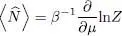
we can integrate over μ (between –∞ and the current value μ , for a fixed value of μ ) to obtain ln Z , and hence the grand potential. From this grand potential, all the other thermodynamic quantities can be calculated, taking the proper derivatives (for example a derivative with respect to β to get the average energy). We shall see an example of this method in § 4-a of the next complement.