Claude Cohen-Tannoudji - Quantum Mechanics, Volume 3

The computation of the average value follows the same steps:

(57)

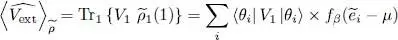
(as in Complement E XV, operator V 1is the one-particle external potential operator).

To complete the calculation of the average value of Ĥ , we now have to compute the trace , the average value of the interaction energy when the system is described by . Using relation (51)we can write this average value as a double trace:

(58)

We now turn to the average value of . The calculation is simplified since is, like Ĥ 0, a one-particle operator; furthermore, the | θi 〉 have been chosen to be the eigenvectors of with eigenvalues – see relation (26). We just replace in (56), Ĥ 0by , and obtain:

(59)

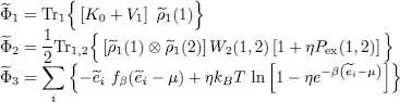
Regrouping all these results and using relation (36), we can write the variational grand potential as the sum of three terms:

(60)

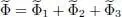
with:

(61)

We now vary the eigenenergies and eigenstates | θk 〉 of to find the value of the density operator that minimizes the average value of the potential. We start with the variations of the eigenstates, which induce no variation of . The computation is actually very similar to that of Complement E XV, with the same steps: variation of the eigenvectors, followed by the demonstration that the stationarity condition is equivalent to a series of eigenvalue equations for a Hartree-Fock operator (a one-particle operator). Nevertheless, we will carry out this computation in detail, as there are some differences. In particular, and contrary to what happened in Complement E XV, the number of states | θi 〉 to be varied is no longer fixed by the particle number N ; these states form a complete basis of the individual state space, and their number can go to infinity. This means that we can no longer give to one (or several) state(s) a variation orthogonal to all the other | θj 〉; this variation will necessarily be a linear combination of these states. In a second step, we shall vary the energies .

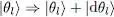
As the eigenstates | θi 〉 vary, they must still obey the orthogonality relations:

(62)

The simplest idea would be to vary only one of them, | θl 〉 for example, and make the change:

(63)

The orthogonality conditions would then require:

(64)

preventing |d θl 〉 from having a component on any ket | θi 〉 other than | θl 〉: in other words, |d θl 〉 and | θl 〉 would be colinear. As | θl 〉 must remain normalized, the only possible variation would thus be a phase change, which does not affect either the density operator (1) or any average values computed with . This variation does not change anything and is therefore irrelevant.

It is actually more interesting to vary simultaneously two eigenvectors, which will be called | θl 〉 and | θm 〉, as it is now possible to give | θl 〉 a component on | θm 〉, and the reverse. This does not change the two-dimensional subspace spanned by these two states; hence their orthogonality with all the other basis vectors is automatically preserved. Let us give the two vectors the following infinitesimal variations (without changing their energies and ):

(65)

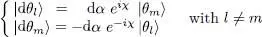
where da is an infinitesimal real number and χ an arbitrary but fixed real number. For any value of χ , we can check that the variation of 〈 θl | θl 〉 is indeed zero (it contains the scalar products 〈 θl | θm 〉 or 〈 θm | θl 〉 which are zero), as is the symmetrical variation of 〈 θm | θm 〉, and that we have: