Claude Cohen-Tannoudji - Quantum Mechanics, Volume 3

(78)

and thus leads to variations of expressions (61)of and . Their sum is:

(79)

where the factor 1/2 in has been canceled since the variations induced by and double each other. Inserting (78)in this relation and using again (74), we get:

(80)

As for , its variation is the sum of a term in coming from the explicit presence of the energies in its definition (61), and a term in . If we let only the energy vary (not taking into account the variations of the distribution function), we get a zero result, since:

(81)

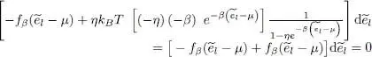
Consequently, we just have to vary by the distribution function, and we get:

(82)

Finally, after simplification by (which, by hypothesis, is different from zero), imposing the variation to be zero leads to the condition:

(83)

This expression does look like the stationarity condition at constant energy (77), but now the subscripts l and m are the same, and a term in is present in the operator.

Introducing a Hartree-Fock operator acting in the single particle state space allows writing the stationarity relations just obtained in a more concise and manageable form, as we now show.

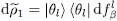
Let us define a temperature dependent Hartree-Fock operator as the partial trace that appears in the previous equations:

(84)

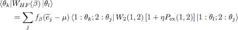
It is thus an operator acting on the single particle 1. It can be defined just as well by its matrix elements between the individual states:

(85)

Equation (77)is valid for any two chosen values l and m , as long as . When l is fixed and m varies, it simply means that the ket:

(86)

is orthogonal to all the eigenvectors | θm 〉 having an eigenvalue different from ; it has a zero component on each of these vectors. As for equation (83), it yields the component of this ket on | θl 〉, which is equal to . The set of | θm 〉 (including those having the same eigenvalue as | θl 〉) form a basis of the individual state space, defined by (26)as the basis of eigenvectors of the individual operator . Two cases must be distinguished:

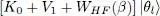
(i) If is a non-degenerate eigenvalue of , the set of equations (77)and (83)determine all the components of the ket [ K0 + V 1+ WHF ( β )]| θl 〉). This shows that | θl 〉 is an eigenvector of the operator K 0+ V 1+ WHF with the eigenvalue .

(ii) If this eigenvalue of is degenerate, relation (77)only proves that the eigen-subspace of , with eigenvalue , is stable under the action of the operator K 0+ V 1+ WHF it does not yield any information on the components of the ket (86)inside that subspace. It is possible though to diagonalize K 0+ V 1+ WHF inside each of the eigen-subspace of , which leads to a new eigenvectors basis | φn 〉, now common to and K 0+ V 1+ WHF .