Claude Cohen-Tannoudji - Quantum Mechanics, Volume 3
Здесь есть возможность читать онлайн «Claude Cohen-Tannoudji - Quantum Mechanics, Volume 3» — ознакомительный отрывок электронной книги совершенно бесплатно, а после прочтения отрывка купить полную версию. В некоторых случаях можно слушать аудио, скачать через торрент в формате fb2 и присутствует краткое содержание. Жанр: unrecognised, на английском языке. Описание произведения, (предисловие) а так же отзывы посетителей доступны на портале библиотеки ЛибКат.

- Название:Quantum Mechanics, Volume 3
- Автор:
- Жанр:
- Год:неизвестен
- ISBN:нет данных
- Рейтинг книги:5 / 5. Голосов: 1
-
Избранное:Добавить в избранное
- Отзывы:
-
Ваша оценка:
Quantum Mechanics, Volume 3: краткое содержание, описание и аннотация
Предлагаем к чтению аннотацию, описание, краткое содержание или предисловие (зависит от того, что написал сам автор книги «Quantum Mechanics, Volume 3»). Если вы не нашли необходимую информацию о книге — напишите в комментариях, мы постараемся отыскать её.
Quantum Mechanics, Volume 3 — читать онлайн ознакомительный отрывок
Ниже представлен текст книги, разбитый по страницам. Система сохранения места последней прочитанной страницы, позволяет с удобством читать онлайн бесплатно книгу «Quantum Mechanics, Volume 3», без необходимости каждый раз заново искать на чём Вы остановились. Поставьте закладку, и сможете в любой момент перейти на страницу, на которой закончили чтение.
Интервал:
Закладка:
Both functions  and
and  increase as a function of μ and, for any given temperature, the total particle number is controlled by the chemical potential. For a large physical system whose energy levels are very close, the orbital part of the discrete sum in (44)can be replaced by an integral. Figure 1of Complement B XVshows the variations of the Fermi-Dirac and Bose-Einstein distributions. We also mentioned that for a boson system, the chemical potential could not exceed the lowest value e 0of the energies el ; when it approaches that value, the population of the corresponding level diverges, which is the Bose-Einstein condensation phenomenon we will come back to in the next complement. For fermions, on the other hand, the chemical potential has no upper boundary, as, whatever its value, the population of states having an energy lower than μ cannot exceed 1.
ϒ. Two particles, distribution functions
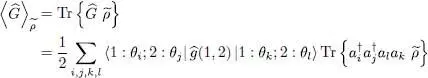
We now consider an arbitrary two-particle operator Ĝ and compute its average value with the density operator  . The general expression of a symmetric two-particle operator is given by relation (C-16) of Chapter XV, and we can write:
(45) 
We follow the same steps as in § 2-a of Complement E XV: we use the mean field approximation to replace the computation of the average value of a two-particle operator by that of average values for one-particle operators. We can, for example, use relation (43)of Complement B XV, which shows that:
(46) 
We then get:
(47) 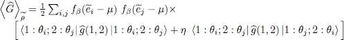
Which, according to (40), can also be written as:
(48) 
where P exis the exchange operator between particles 1 and 2. Since:
(49) 
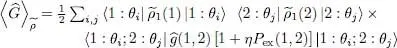
and as the operators  (1) and (2) are diagonal in the basis | θi 〉, we can write the right-hand side of (48)as:
(50) 
which is simply a (double) trace on two particles 1 and 2. This leads to:
(51) 
As announced above, the average value of the two-particle operator Ĝ can be expressed, within the Hartree-Fock approximation, in terms of the one-particle reduced density operator (1); this relation is not linear.
Comment:
The analogy with the computations of Complement Exv becomes obvious if we regroup its equations (57)and (58)and write:
(52) 
Replacing W 2(1, 2) by G , we get a relation very similar to (51), except for the fact that the projectors PN must be replaced by the one-particle operators . In § 3-d, we shall come back to the correspondence between the zero and non-zero temperature results.
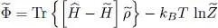
2-c. Variational grand potential
We now have to compute the grand potential  written in (30). As the exponential form (28)for the trial operator makes it easy to compute ln , we see that the terms in μ
  cancel out, and we get:
(53) 
We now have to compute the average energy, with the density operator , of the difference between the Hamiltonians Ĥ and  respectively defined by (1)and (25).
We first compute the trace:
(54) 
starting with the kinetic energy contribution Ĥ 0in (1). We call K 0the individual kinetic energy operator:
(55) 
( m is the particle mass). Equality (43)applied to Ĥ 0yields the average kinetic energy when the system is described by :
(56) 
This result is easily interpreted; each individual state contributes its average kinetic energy, multiplied by its population.
Читать дальшеИнтервал:
Закладка:
Похожие книги на «Quantum Mechanics, Volume 3»
Представляем Вашему вниманию похожие книги на «Quantum Mechanics, Volume 3» списком для выбора. Мы отобрали схожую по названию и смыслу литературу в надежде предоставить читателям больше вариантов отыскать новые, интересные, ещё непрочитанные произведения.


Обсуждение, отзывы о книге «Quantum Mechanics, Volume 3» и просто собственные мнения читателей. Оставьте ваши комментарии, напишите, что Вы думаете о произведении, его смысле или главных героях. Укажите что конкретно понравилось, а что нет, и почему Вы так считаете.