Claude Cohen-Tannoudji - Quantum Mechanics, Volume 3

4 4 If in (15)we set , we see that obeys the differential equation obtained by replacing λ(t) by in (15). If we simply choose for α(t) the integral over time of the function λ(t), this constant will disappear from the differential equation.

5 5 The same argument as above, but starting from the variation δS — iδ′S, would lead to the complex conjugate of (8), and hence to the same equation.

1 1 Variational principle 1-a Notation, statement of the problem 1-b A useful inequality 1-c Minimization of the thermodynamic potential

2 2 Approximation for the equilibrium density operator …. 2-a Trial density operators 2-b Partition function, distributions 2-c Variational grand potential 2-d Optimization

3 3 Temperature dependent mean field equations 3-a Form of the equations 3-b Properties and limits of the equations 3-c Differences with the zero-temperature Hartree-Fock equations (fermions) 3-d Zero-temperature limit (fermions) 3-e Wave function equations

Understanding the thermal equilibrium of a system of interacting identical particles is important for many physical problems: conductor or semiconductor electronic properties, liquid Helium or ultra-cold gas properties, etc. It is also essential for studying phase transitions, various and multiple examples of which occur in solid and liquid physics: spontaneous magnetism appearing below a certain temperature, changes in electrical conduction, and many others. However, even if the Hamiltonian of a system of identical particles is known, calculation of the equilibrium properties cannot, in general, be carried to completion: these calculations present real difficulties in the handling of state vectors and interaction operators, where non-trivial combinations of creation and annihilation operators occur. One must therefore use one or several approximations. The most common one is probably the mean field approximation, which, as we saw in Complement E XV, is the base of the Hartree-Fock method. In that complement, we showed, in terms of state vectors, how this method could be used to obtain approximate values for the energy levels of a system of interacting particles. As we consider here the more complex problem of thermal equilibrium, which must be treated in terms of density operators, we show how the Hartree-Fock method can be extended to this more general case.

We are going to see that, thanks to this approach, one can obtain compact formulas for an approximate value of the density operator at thermal equilibrium, in the framework of the grand canonical ensemble. The equations to be solved are fairly similar 1 to those of Complement E XV. The Hartree-Fock method also gives a value of the thermodynamic grand potential, which leads directly to the pressure of the system. The other thermodynamic quantities can then be obtained via partial derivatives with respect to the equilibrium parameters (volume, temperature, chemical potential, eventually external applied field, etc. – see Appendix VI). It is clearly a powerful method even though it still is an approximation as the particles interactions are treated via a mean field approach where certain correlations are not taken into account. Furthermore, for bosons, it can only be applied to physical systems far from Bose-Einstein condensation; the reasons for this limitation will be discussed in detail in § 4-a of Complement H XV.

Once we have recalled the notation and a few generalities, we shall establish (§ 1) a variational principle that applies to any density operator. It will allow us to search in any family of operators for the one closest to the density operator at thermal equilibrium. We will then introduce (§ 2) a family of trial density operators whose form reflects the mean field approximation; the variational principle will help us determine the optimal operator. We shall obtain Hartree-Fock equations for a non-zero temperature, and study some of their properties in the last section (§ 3). Several applications of these equations will be presented in Complement H XV.

The general idea and the structure of the computations will be the same as in Complement E XV, and we keep the same notation: we establish a variational condition, choose a trial family, and then optimize the system description within this family. This is why, although the present complement is self-contained, it might be useful to first read Complement E XV.

In order to use a certain number of general results of quantum statistical mechanics (see Appendix refappend-6 for a more detailed review), we first introduce the notation.

We assume the Hamiltonian is of the form:

(1)

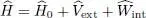
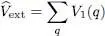
which is the sum of the particles’ kinetic energy Ĥ 0, their coupling energy with an external potential:

(2)

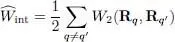
and their mutual interaction , which can be expressed as:

(3)

We are going to use the “grand canonical” ensemble ( Appendix VI, § 1-c), where the particle number is not fixed, but takes on an average value determined by the chemical potential μ . In this case, the density operator ρ is an operator acting in the entire Fock space εF (where N can take on all the possible values), and not only in the state space εN for N particles (which is is more restricted since it corresponds to a fixed value of N ). We set, as usual:

(4)

where kB is the Boltzmann constant and T the absolute temperature. At the grand canonical equilibrium, the system density operator depends on two parameters, β and the chemical potential μ , and can be written as:

(5)

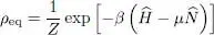
with the relation that comes from normalizing to 1 the trace of ρ eq:

(6)

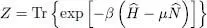
The function Z is called the “grand canonical partition function” (see Appendix VI, § 1-c). The operator associated with the total particle number is defined in (B-17) of Chapter XV. The temperature T and the chemical potential μ are two intensive quantities, respectively conjugate to the energy and the particle number.