Claude Cohen-Tannoudji - Quantum Mechanics, Volume 3

Let us write for example that , which means the right-hand side of the second line in (13)must be zero. As the time evolution between t 0and t 1of the bra is arbitrary, this condition imposes this bra multiplies a zero-value ket, at all times. Consequently, the ket must obey the equation:

(15)

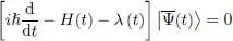
which is none other than the Schrödinger equation associated with the Hamiltonian H ( t ) + λ ( t ).

Actually, λ ( t ) simply introduces a change in the origin of the energies and this only modifies the total phase 4 of the state vector , which has no physical effect. Without loss of generality, this Lagrange factor may therefore be ignored, and we can set:

(16)

A necessary condition 5 for the stationarity of S is that obey the Schrödinger equation (8)– or be physically equivalent (i.e. equal to within a global time-dependent phase factor) to a solution of this equation. Conversely, assume is a solution of the Schrödinger equation, and give this ket a variation as in (11). It is then obvious from the second line of (13)that is zero. As for , an integration by parts over time shows that it is the complex conjugate of , and therefore also equal to zero. The functional S is thus stationary in the vicinity of any exact solution of the Schrödinger equation.

Suppose we choose any variational family of normalized kets , but which now includes a ket for which S is stationary. A simple example is the case where is a family that contains the exact solution of the Schrödinger equation; according to what we just saw, this exact solution will make S stationary, and conversely, the ket that makes S stationary is necessarily . In this case, imposing the variation of S to be zero allows identifying, inside the family , the exact solution we are looking for. If we now change the family continuously from to , in general will no longer contain the exact solution of the Schrödinger equation. We can however follow the modifications at all times of the values of the ket . Starting from an exact solution of the equation, this ket progressively changes, but, by continuity, will stay in the vicinity of this exact solution if stays close to . This is why annulling the variation of S in the family is a way of identifying a member of that family whose evolution remains close to that of a solution of the Schrödinger equation. This is the method we will follow, using the Fock states as a particular variational family.

If the Hamiltonian H is time-independent, one can look for time-independent kets to make the functional S stationary. The function to be integrated in the definition of the functional S also becomes time-independent, and we can write S as:

(17)

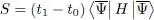
Since the two times t 0and t 1are fixed, the stationarity of S is equivalent to that of the diagonal matrix element of the Hamiltonian . We find again the stationarity condition of the time-independent variational method (Complement E XI), which appears as a particular case of the more general method of the time-dependent variations. Consequently, it is not surprising that the Hartree-Fock methods, time-dependent or not, lead to the same Hartree-Fock potential, as we now show.

The family of the state vectors we consider is the set of Fock kets defined in (1). We first compute the function to be integrated in the functional (10)when |Ψ( t )〉 takes the value .