Claude Cohen-Tannoudji - Quantum Mechanics, Volume 3

Let us introduce a general variational principle; using the stationarity of a functional S of the state vector Ψ( t )〉, it will yield the time-dependent Schrödinger equation.

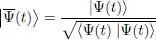
Consider an arbitrarily given Hamiltonian H ( t ). We assume the state vector |Ψ( t )〉 to have any time dependence, and we note the ket physically equivalent to |Ψ( t )〉, but with a constant norm:

(6)

The functional S of is defined as 1 :

(7)

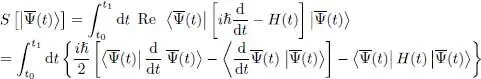
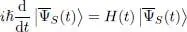
where t 0and t 1are two arbitrary times such that t 0< t 1. In the particular case where the chosen is equal to a solution of the Schrödinger equation:

(8)

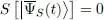
the bracket on the first line of (7)obviously cancels out and we have:

(9)

Integrating by parts the second term 2 of the bracket in the second line of (7), we get the same form as the first term in the bracket, plus an already integrated term. The final result is then:

(10)

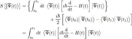
where we have used in the second line the fact that the norm of always remains equal to unity. This expression for S is similar to the initial form (7), but without the real part.

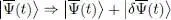
Suppose now has an arbitrary time dependence between t 0and t 1, while keeping its norm constant, as imposed by (6); the functional then takes a certain value S , a priori different from zero. Let us see under which conditions S will be stationary when changes by an infinitely small amount :

(11)

For what follows, it will be convenient to assume that the variation is free; we therefore have to ensure that the norm of remains constant, equal to unity 3 . We introduce Lagrange multipliers (Appendix V) λ( t ) to control the square of the norm at every time between t 0and t 1, and we look for the stationarity of a function where the sum of constraints has been added. This sum introduces an integral, and we the function in question is:

(12)

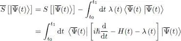
where λ( t ) is a real function of the time t .

The variation of to first order is obtained by inserting (11)in (10). It yields the sum of a first term containing the ket and of another containing the bra :

(13)

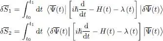
We now imagine another variation for the ket:

(14)

which yields a variation of ; in this second variation, the term in becomes , whereas the term in becomes . Now, if the functional is stationary in the vicinity of , the two variations and are necessarily zero, as are also and . In those combinations, only terms in appear for the first one, and in for the second; consequently they must both be zero. As a result, we can write the stationarity conditions with respect to variations of the bra and the ket separately.