Claude Cohen-Tannoudji - Quantum Mechanics, Volume 3

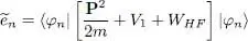
The variational energy can be computed in the same way as in § 1-e. Multiplying on the left equation (77)by the bra 〈 φn |, we get:

(79)

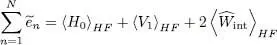
After summing over the subscript n , we obtain:

(80)

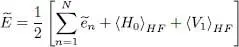
Taking into account (51), (53), and (61), we get:

(81)

where the particle interaction energy is counted twice. To compute the energy , we can eliminate between (26)and this relation and we finally obtain:

(82)

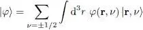
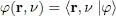
Assume the fermions we are studying are particles with spin 1/2, electrons for example. The basis {| r〉} of the individual states used in § 1 must be replaced by the basis formed with the kets {| r, ν )}, where ν is the spin index, which can take 2 distinct values noted ±1/2, or more simply ±. To the summation over d 3 r we must now add a summation over the 2 values of the index spin ν . A vector | φ 〉 in the individual state space is now written:

(83)

with:

(84)

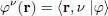
The variables rand ν play a similar role but the first one is continuous whereas the second is discrete. Writing them in the same parenthesis might hide this difference, and we often prefer noting the discrete index as a superscript of the function φ and write:

(85)

Let us build an N particle variational state from N orthonormal states , with n =1, 2,.. , N . Each of the describes an individual state including the spin and position variables; the first N +values of νn ( n = 1,2,.. N +) are equal to +1/2, the last N –are equal to –1/2, with N ++ N –= N (we assume N +and N -are fixed for the moment but we may allow them to vary later to enlarge the variational family). In the space of the individual states, we introduce a complete basis whose first N kets are the , but where the subscript k varies from 1 to infinity 7 .

We assume the matrix elements of the external potential V 1to be diagonal for ν ; these two diagonal matrix elements can however take different values , which allows including the eventual presence of a magnetic field coupled with the spins. We also assume the particle interaction W 2(1,2) to be independent of the spins, and diagonal in the position representation of the two particles, as is the case, for example, for the Coulomb interaction between electrons. With these assumptions, the Hamiltonian cannot couple states having different particle numbers N +and N –.

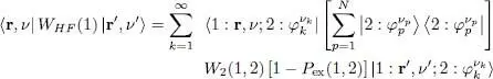
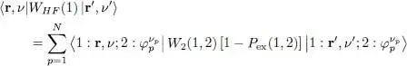
Let us see what the general Hartree-Fock equations become in the {| r, ν 〉} representation. In this representation, the effect of the kinetic and potential operators are well known. We just have to compute the effect of the Hartree-Fock potential WHF . To obtain its matrix elements, we use the basis 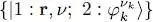to write the trace in (60):

(86)

As the right-hand side includes the scalar product 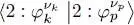which is equal to δkp , the sum over k disappears and we get:

(87)

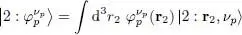
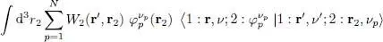
(i) We first deal with the direct term contribution, hence ignoring in the bracket the term in P ex(1, 2). We can replace the ket by its expression:

(88)

As the operator is diagonal in the position representation, we can write:

(89)

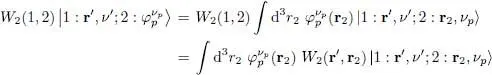
The direct term of (87)is then written:

(90)

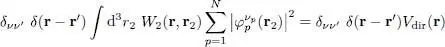
where the scalar product of the bra and the ket is equal to 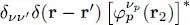. We finally obtain:

(91)