Claude Cohen-Tannoudji - Quantum Mechanics, Volume 3

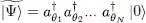
We assume as before that the N -particle variational ket is written as:

(47)

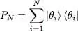
This ket is derived from N individual orthonormal kets | θk 〉, but these kets can now describe particles having an arbitrary spin. Consider the orthonormal basis {| θk 〉} of the one-particle state space, in which the set of | θi 〉 ( i = 1, 2, … N ) was completed by other orthonormal states. The projector PN onto the subspace is the sum of the projections onto the first N kets | θi 〉:

(48)

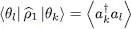
This is simply the one-particle density operator defined in § B-4 of Chapter XV(normalized by a trace equal to the particle number N and not to one), as we now show. Relation (B-24) of that chapter can be written in the | θk 〉 basis:

(49)

where the average value is taken in the quantum state (47). In this kind of Fock state, the average value is different from zero only when the creation operator reconstructs the population destroyed by the annihilation operator, hence if k = l , in which case it is equal to the population nk of the individual states | θk 〉. In the variational ket (47), all the populations are zero except for the first N states | θi 〉 ( i = 1, 2, … N ), where they are equal to one. Consequently, the one-particle density operator is represented by a matrix, diagonal in the basis | θi 〉, and whose N first elements on the diagonal are all equal to one. It is indeed the matrix associated with the projector PN , and we can write:

(50)

As we shall see, all the average values useful in our calculation can be simply expressed as a function of this operator.

We now evaluate the different terms included in the average energy, starting with the terms containing one-particle operators.

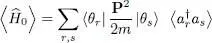
Using relation (B-12) of Chapter XV, we obtain for the average kinetic energy 〈 Ĥ 0〉:

(51)

The same argument as that for the evaluation of the matrix elements (49)shows that the average value in the state (47)is only different from zero if r = s ; in that case, it is equal to one when r ≤ N , and to zero otherwise. This leads to:

(52)

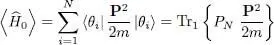
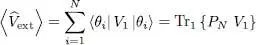
The subscript 1 was added to the trace to underline the fact that this trace is taken in the one-particle state space and not in the Fock space. The two operators included in the trace only act on that same particle, numbered arbitrarily 1; the subscript 1 could obviously be replaced by the subscript of any other particle, since they all play the same role. The average potential energy coming from the external potential is computed in a similar way and can be written as:

(53)

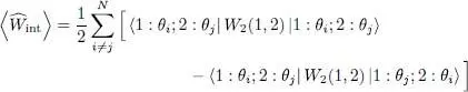
The average interaction energy can be computed using the general expression (C-16) of Chapter XVfor any two-particle operator, which yields:

(54)

For the average value in the Fock state to be different from zero, the operator must leave unchanged the populations of the individual states | θn 〉 and | θq 〉. As in § C-5-b of Chapter XV, two possibilities may occur: either r = n and s = q (the direct term), or r = q and s = n (the exchange term). Commuting some of the operators, we can write:

(55)

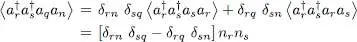
where nr and ns are the respective populations of the states | θr 〉 and | θs 〉. Now these populations are different from zero only if the subscripts r and s are between 1 and N , in which case they are equal to 1 (note also that we must have r ≠ s to avoid a zero result). We finally get 5 :

(56)

(the constraint i ≠ j may be ignored since the right-hand side is equal to zero in this case). Here again, the subscripts 1 and 2 label two arbitrary, but different particles, that could have been labeled arbitrarily. We can therefore write:

(57)

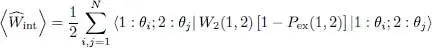
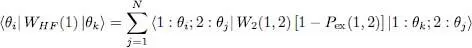
where P ex(1,2) is the exchange operator between particle 1 and 2 (the transposition which permutes them). This result can be written in a way similar to (53)by introducing a “Hartree-Fock potential” WHF , similar to an external potential acting in the space of particle 1; this potential is defined as the operator having the matrix elements:

(58)