Claude Cohen-Tannoudji - Quantum Mechanics, Volume 3
Здесь есть возможность читать онлайн «Claude Cohen-Tannoudji - Quantum Mechanics, Volume 3» — ознакомительный отрывок электронной книги совершенно бесплатно, а после прочтения отрывка купить полную версию. В некоторых случаях можно слушать аудио, скачать через торрент в формате fb2 и присутствует краткое содержание. Жанр: unrecognised, на английском языке. Описание произведения, (предисловие) а так же отзывы посетителей доступны на портале библиотеки ЛибКат.

- Название:Quantum Mechanics, Volume 3
- Автор:
- Жанр:
- Год:неизвестен
- ISBN:нет данных
- Рейтинг книги:5 / 5. Голосов: 1
-
Избранное:Добавить в избранное
- Отзывы:
-
Ваша оценка:
Quantum Mechanics, Volume 3: краткое содержание, описание и аннотация
Предлагаем к чтению аннотацию, описание, краткое содержание или предисловие (зависит от того, что написал сам автор книги «Quantum Mechanics, Volume 3»). Если вы не нашли необходимую информацию о книге — напишите в комментариях, мы постараемся отыскать её.
Quantum Mechanics, Volume 3 — читать онлайн ознакомительный отрывок
Ниже представлен текст книги, разбитый по страницам. Система сохранения места последней прочитанной страницы, позволяет с удобством читать онлайн бесплатно книгу «Quantum Mechanics, Volume 3», без необходимости каждый раз заново искать на чём Вы остановились. Поставьте закладку, и сможете в любой момент перейти на страницу, на которой закончили чтение.
Интервал:
Закладка:
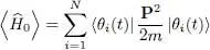
For the term in H ( t ), the calculation is identical to the one we already did in § 1-b of Complement E XV. We first add to the series of orthonormal states | θi ( t )〉 with i = 1, 2, …, N other orthonormal states | θi ( t )〉 with i = N + 1, N + 2, …, to obtain a complete orthonormal basis in the space of individual states. Using this basis, we can express the one-particle and two-particle operators according to relations (B-12) and (C-16) of Chapter XV. This presents no difficulty since the average values of creation and annihilation operator products are easily obtained in a Fock state (they only differ from zero if the product of operators leaves the populations of the individual states unchanged). Relations (52), (53) and (57) of Complement E XVare still valid when the | θi 〉 become time-dependent. We thus get for the average kinetic energy:
(18) 
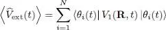
for the external potential energy:
(19) 
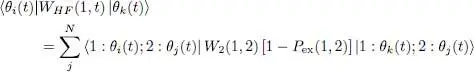
and for the interaction energy:
(20) 
3-b. Hartree-Fock potential
We recognize in (20)the diagonal element ( i = k ) of the Hartree-Fock potential operator WHF (1, t ) whose matrix elements have been defined in a general way by relation (58) of Complement E XV:
(21) 
We also noted in that complement E XVthat WHF (1, t ) is a Hermitian operator.
It is often handy to express the Hartree-Fock potential using a partial trace:
(22) 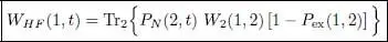
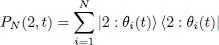
where PN is the projector onto the subspace spanned by the N kets | θi ( t )〉:
(23) 
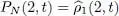
As we have seen before, this projector is actually nothing bu the one-particle reduced density operator  normalized by imposing its trace to be equal to the total particle number N :
(24) 
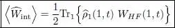
The average value of the interaction energy can then be written as:
(25) 
3-c. Time derivative
As for the time derivative term, the function it contains can be written as:
(26) 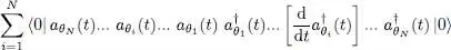
In this summation, all terms involving the individual states j other than the state i (which is undergoing the derivation) lead to an expression of the type:
(27) 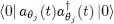
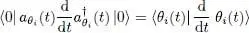
which equals 1 since this expression is the square of the norm of the state  , which is simply the Fock state | nj = 1〉. As for the state i , it leads to a factor written in the form of a scalar product in the one-particle state space:
(28) 
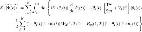
3-d. Functional value
Regrouping all these results, we can write the value of the functional S in the form:
(29) 
4. Equations of motion
We now vary the ket | θk ( t )〉 according to:
(30) 
As in complement E XV, we will only consider variations | δθk ( t )〉 that lead to an actual variation of the ket  ; those where | δθk ( t )〉 is proportional to one of the occupied states | θl ( t )〉 with l ≤ N yield no change for (or at the most to a phase change) and are thus irrelevant for the value of S . As we did in relations (32)or (69) of Complement E XV, we assume that:
(31) 
where δf ( t ) is an infinitesimal time-dependent function.
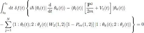
The computation is then almost identical to that of § 2-b in Complement E XV. When | θk ( t )〉 varies according to (31), all the other occupied states remaining constant, the only changes in the first line of (29)come from the terms i = k . In the second line, the changes come from either the i = k terms, or the j = k terms. As the W 2(1,2) operator is symmetric with respect to the two particles, these variations are the same and their sum cancels the 1/2 factor. All these variations involve terms containing either the ket eiχ | δθk ( t )〉, or the bra 〈 δθk ( t )| e–iχ . Now their sum must be zero for any value of χ, and this is only possible if each of the terms is zero. Inserting the variation (31)of | θk ( t )〉, and canceling the term in e–iχ leads to the following equality:
(32) 
Интервал:
Закладка:
Похожие книги на «Quantum Mechanics, Volume 3»
Представляем Вашему вниманию похожие книги на «Quantum Mechanics, Volume 3» списком для выбора. Мы отобрали схожую по названию и смыслу литературу в надежде предоставить читателям больше вариантов отыскать новые, интересные, ещё непрочитанные произведения.


Обсуждение, отзывы о книге «Quantum Mechanics, Volume 3» и просто собственные мнения читателей. Оставьте ваши комментарии, напишите, что Вы думаете о произведении, его смысле или главных героях. Укажите что конкретно понравилось, а что нет, и почему Вы так считаете.