Claude Cohen-Tannoudji - Quantum Mechanics, Volume 3

As we recognize in the function to be integrated the Hartree-Fock potential operator WHF (1, t ) defined in (21), we can write:

(33)

with l > N .

As the choice of the function δf ( t ) is arbitrary, for expression (33)to be zero for any δf ( t ) requires the function inside the curly brackets to be zero at all times t . Stationarity therefore requires the ket:

(34)

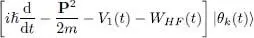
to have no components on any of the non-occupied states | θl ( t )〉 with ( l > N ). In other words, stationarity will be obtained if, for all values of k & between 1 and N , we have:

(35)

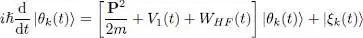
where | ξk ( t )〉 is any linear combination of the occupied states | θl ( t )〉 ( l < N ). As we pointed out at the beginning of § 4, adding to one of the | θk ( t )〉 a component on the already occupied individual states has no effect on the Af-particle state (aside from an eventual change of phase), and therefore does not change the value of S ; consequently, the stationarity of this functional does not depend on the value of the ket | ξk ( t )〉, which can be any ket, for example the zero ket.

Finally, if the | θn ( t )〉 are equal to the solutions | φn ( t )〉 of the N equations:

(36)

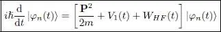
the functional S is indeed stationary for all times. Furthermore, as we saw in Complement E xvthat WHF ( t ) is Hermitian, so is the operator on the right-hand side of (36). Consequently, the N kets | φn ( t )〉 follow an evolution similar to the usual Schrödinger evolution, described by a unitary evolution operator (Complement F III). Such an operator does not change either the norm nor the scalar products of the kets: if the kets | φn ( t )〉x initially formed an orthonormal set, this remains true at any later time. The whole calculation just presented is thus consistent; in particular, the norm of the N -particle state vector is constant over time.

Relations (36)are the time-dependent Hartree-Fock equations. Introducing the one-particle mean field operator allowed us not only to compute the stationary energy levels, but also to treat time-dependent problems.

Let us return to the particular case of fermions all having the same spin state, as in § 1 of Complement E XV. We can then write the Hartree-Fock equations in terms of the wave functions as:

(37)

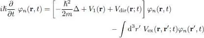
using definitions of (46) of that complement for the direct and exchange potentials, which are now time-dependent. There is obviously a close relation between the Hartree-Fock equations, whether they are time-dependent or not.

As encountered in the search for a ground state with the time-independent Hartree-Fock equations, there is a strong similarity between equations (36)and an ordinary Schrödinger equation for a single particle. Here again, an exact solution of these equations is generally not possible, and we must use successive approximations. Assume for example that the external time-dependent potential V 1( i ) is zero until time t0 and that for t < t 0, the physical system is in a stationary state. With the time-independent Hartree-Fock method we can compute an approximate value for this state and hence a series of initial values for the individual states | φn ( t 0)〉. This determines the initial Hartree-Fock potential. Between time t 0to and a slightly later time t 0+ Δ t , the evolution equation (36)describes the effect of the external potential V 1( t ) on the individual kets, and allows obtaining the | φn ( t 0+ Δ t )〉. We can then compute a new value for the Hartree-Fock potential, and use it to extend the computation of the evolution of the | φn ( t )〉 until a later time t 0+ 2Δ t . Proceeding step by step, we can obtain this evolution until the final time t 1. For the approach to be precise, Δ t must be small enough for the Hartree-Fock potential to change only slightly from one time step to another.

Another possibility is to proceed as in the search for the stationary states. We start from a first family of orthonormal kets, now time-dependent, and which are not too far from the expected solution over the entire time interval; we then try to improve it by successive iterations. Inserting in (21)the first series of orthonormal trial functions, we get a first approximation of the Hartree-Fock potential and its associated dynamics. We then solve the corresponding equation of motion, with the same initial conditions at t = t 0, which yields a new series of orthonormal functions. Using again (21), we get a value for the Hartree-Fock potential, a priori different from the previous one. We start the same procedure anew until an acceptable convergence is obtained.

Applications of this method are quite numerous, in particular in atomic, molecular, and nuclear physics. They allow, for example, the study of the electronic cloud oscillations in an atom, a molecule or a solid, placed in an external time-dependent electric field (dynamic polarisability), or the oscillations of nucleons in their nucleus. We mentioned in the conclusion of Complement E xvthat the time-independent Hartree-Fock method is sometimes replaced by the functional density method; this is also the case when dealing with time-dependent problems.

In concluding this complement we underline the close analogy between the Hartree-Fock theory and a time-independent or a time-dependent mean field theory. In both cases the same Hartree-Fock potential operators come into play. Even though they are the result of an approximation, these operators have a very large range of applicability.

1 1 The notation where the differential operator d/dt is written between a bra and a ket means that the operator takes the derivative of the ket that follows (and not of the bra just before).

2 2 If we integrate by parts the first term rather than the second, we get the complex conjugate of equation (10), which brings no new information.

3 3 For the normalization of to be conserved to first order, it is necessary (and sufficient) for the scalar product to be zero or purely imaginary. If this is the case, the Lagrangian multiplier λ(t) is not needed