Claude Cohen-Tannoudji - Quantum Mechanics, Volume 3

(10)

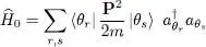
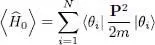
where the two summations over r and s range from 1 to D . The average value in of the kinetic energy can then be written:

(11)

which contains the scalar product of the ket:

(12)

by the bra:

(13)

Note however that in the ket, the action of the annihilation operator aθs yields zero unless it acts on a ket where the individual state is already occupied; consequently, the result will be different from zero only if the state | θS 〉 is included in the list of the N states | θ 1〉, | θ 2〉, ….| θN 〉. Taking the Hermitian conjugate of (13), we see that the same must be true for the state | θr 〉, which must be included in the same list. Furthermore, if r ≠ s the resulting kets have different occupation numbers, and are thus orthogonal. The scalar product will therefore only differ from zero if r = s , in which case it is simply equal to 1. This can be shown by moving to the front the state | θr 〉 both in the bra and in the ket; this will require two transpositions with two sign changes which cancel out, or none if the state | θr 〉 was already in the front. Once the operators have acted, the bra and the ket correspond to exactly the same occupied states and their scalar product is 1. We finally get:

(14)

Consequently, the average value of the kinetic energy is simply the sum of the average kinetic energy in each of the occupied states | θi 〉.

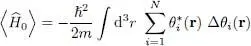
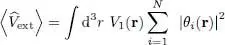
For spinless particles, the kinetic energy operator is actually a differential operator – ħ 2Δ/2 m acting on the individual wave functions. We therefore get:

(15)

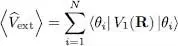
As the potential energy is also a one-particle operator, its average value can be computed in a similar way. We obtain:

(16)

that is, for spinless particles:

(17)

As before, the result is simply the sum of the average values associated with the individual occupied states.

The average value of the interaction energy in the state has already been computed in § C-5 of Chapter XV. We just have to replace, in the relations (C-28) as well as (C-32) to (C-34) of that chapter, the ni by 1 for all the occupied states | θi 〉, by zero for the others, and to rename the wave functions ui ( r) as θi ( r). We then get:

(18)

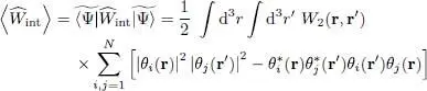
We have left out the condition i ≠ j no longer useful since the i = j terms are zero. The second line of this equation contains the sum of the direct and the exchange terms.

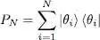
The result can be written in a more concise way by introducing the projector PN over the subspace spanned by the N kets | θi 〉:

(19)

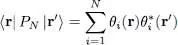
Its matrix elements are:

(20)

This leads to:

(21)

Comment:

The matrix elements of PN are actually equal to the spatial non-diagonal correlation function G 1( r, r′), which will be defined in Chapter XVI(§ B-3-a). This correlation function can be expressed as the average value of the product of field operators Ψ( r):

(22)

For a system of N fermions in the states | θ 1〉, | θ 2〉, ..,| θN 〉, we can write:

(23)

Inserting this relation in (18)we get:

(24)

Comparison with relation (C-28) of Chapter XV, which gives the same average value, shows that the right-hand side bracket contains the two-particle correlation function G 2( r, r′). For a Fock state, this function can therefore be simply expressed as two products of one-particle correlation functions at two points:

(25)