Claude Cohen-Tannoudji - Quantum Mechanics, Volume 3

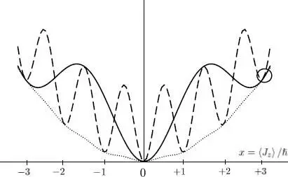
Figure 3: Plots of the energy of a rotating repulsive boson system, in a coherent superposition of the state l and the state l′, as a function of its average angular momentum 〈 Jz 〉 , expressed in units of ħ. The lower dotted curve corresponds to the case where l′ = l — 1 and the interaction constant g is small (almost ideal gas). The potential energy is then negligible and the total energy presents a single minimum in 〈 Jz 〉 = 0. Consequently, whatever the initial rotational state of the fluid, it will relax to a motionless state l = 0 without having to go over any energy barrier, and its rotational kinetic energy will dissipate: it behaves as a normal fluid. The other two curves correspond to a much larger value of g - therefore, according to (39) to a much higher value of c. The dashed curve still corresponds to a superposition of the rotational states l and l′ = l — 1, and the solid line to the direct superposition of the state l = 3 (shown with a circle in the figure) and the ground state l ′ = 0. The solid line curve presents the smallest barrier, hence determining the metastability of the current .

The higher the coupling constant g, the more l states presenting a minimum in the potential energy appear. They correspond to flow velocities in the torus that are smaller than the critical velocity. To go from the rotational state l = 1 to the motionless state l = 0, the system must go over a macroscopic energy barrier, which only occurs with a probability so small it can be considered equal to zero. The rotational current is therefore permanent, lasting for years, and the system is said to be superfluid. On the other hand, the states with higher values of l, for which the curve presents no minima, correspond to a normal fluid, whose rotation can slow down because of the viscosity (dissipation of the kinetic energy into heat) .

Our argument remained qualitative for several reasons. To begin with, we showed the existence for the fluid of a critical velocity vc , of the order of c , without giving its precise value. It would require a more detailed study of the potential curves such as the ones plotted in Figure 3, to obtain the precise values of the parameters for which the potential barrier appears or disappears. We also limited ourselves to simple geometries that could be described by a single variable φ not taking into account other possible deformations of the wave function. Various situations could occur, such as the creation of vortices or more complex processes, which would require a more elaborate mathematical treatment. In other words, we would have to take into account the existence of other relaxation channels for the moving fluid to come to rest, and look for the one leading to the lowest potential barrier, thereby determining the lifetime of the superfluid current.

There is, however, a more general way to address the problem, which shows that our basic conclusions are not limited to the particular case we have studied. It is based on the topological aspects of the wave function phase. When this phase varies by 2 l π as we go around the torus, it expresses a topological property characterized by the winding number l , which is an integer and cannot vary continuously. This is why, as long as the phase is well defined everywhere – i.e. as long as the wave function does not go to zero – we cannot go continuously from l to l ± 1. We already saw this in the particular example of the wave function (63): when the modulus of cl ( t ) varies in time from 1 to 0, while the modulus of cl′ ( t ) does the opposite, we necessarily went through a situation where the wave function went to zero through interference, in a plane corresponding to a certain value of φ ; but the phase of the wave function is undetermined in this plane, and as we cross it, the phase undergoes a discontinuous jump. Now the canceling of the wave function of a great number of condensed bosons means the density must also be zero at that point, hence larger in other points of space. This spatial density variation introduces an energy increase, due to the finite compressibility of the fluid (as we saw in § 3-b, the energy increase in the high density regions is larger than the energy decrease in low density regions). This means there is an energy barrier opposing the change in the number of turns l of the phase. The height of this barrier must now be compared with the kinetic energy variation. As seen above, there is a drastic change in the flow regime, depending on whether the fluid velocity is smaller or larger than a certain critical velocity vc . In the first case, superfluidity allows a current to flow without dissipation, lasting practically indefinitely. In the second, no energy consideration opposes dissipation, and the rotation slows down progressively, as in an ordinary liquid.

The essential idea to remember is that superfluidity comes from the repulsive interactions, and for two reasons. First of all, they explain the presence of the energy barrier, responsible for the metastability. The second reason, even more essential, is that the repulsion between bosons constantly tends to put all the fluid particles in the same quantum state – see § 4-c of Complement C XV; thanks to this property, we were able to characterize the intermediate rotational states by a very simple wave function (63). This implies that the quantum fluid can only occupy a very limited number of states, compared to a situation where the particles would be distinguishable. Consequently, it has a hard time dissipating its kinetic energy into heat, as a classical fluid would do, and it therefore maintains its rotation over such long times that a slowing down is practically impossible to observe.

1 1 It is a “total derivative” term (the derivative describing, in a fluid, the motion of each particle). As the velocity field has a zero curl according to (51), a simple vector analysis calculation shows this term to be equal to m(v · ▽)v; it can therefore be accounted for by replacing on the left-hand side of (57)the partial derivative ∂/∂t by the total derivative d/dt = ∂/∂t + v · ∇.

2 2 The quantum potential is still present for a single particle, since making g = 0 in (57)does not change this potential. For g = 0, the Gross-Pitaevskii equation simply reduces to the standard Schrödinger equation, valid for a single particle.

3 3 or not at all, if we suppose the functions ul(r, z) and ul′(r, z) to be equal.

4 4 When several relaxation channels are present, the one associated with the lowest barrier mainly determines the time evolution.

1 1 Foundation of the method 1-a Trial family and Hamiltonian 1-b Energy average value 1-c Optimization of the variational wave function 1-d Equivalent formulation for the average energy stationarity 1-e Variational energy 1-f Hartree-Fock equations

2 2 Generalization: operator method 2-a Average energy 2-b Optimization of the one-particle density operator 2-c Mean field operator 2-d Hartree-Fock equations for electrons 2-e Discussion

Computing the energy levels of a system of N electrons, interacting with each other through the Coulomb force, and placed in an external potential V 1( r) is a very important problem in physics and chemistry. It is encountered in the determination of the energy levels of atoms (in which case the external potential for the electrons 1 is the Coulomb potential created by the nucleus – Zq 2/4π ε 0 r ), or of molecules as well, or of electrons in a solid (submitted to a periodic potential), or in an aggregate or a nanocristal, etc. It is a problem where two ingredients simultaneously play an essential role: the fermionic character of the electrons, which forbids them to occupy the same individual state, and the effects of their mutual interactions. Ignoring the Coulomb repulsion between electrons would make the calculation fairly simple, and similar to that of § 1 in Complement C XIV, concerning free fermions in a box; the free plane wave individual states would have to be replaced by the energy eigenstates of a single particle placed in the potential V 1( r). This would lead to a 3-dimensional Schrodinger equation, which can be solved with very good precision, although not necessarily analytically.