Claude Cohen-Tannoudji - Quantum Mechanics, Volume 3

Let us compute the spatial and time evolution of the particle density n ( r, t) when δφ ( r, t ) obeys relation (28). The particle density at each point rof space is the sum of the densities associated with each particle, that is N times the squared modulus of the wave function φ ( r, t ). To first-order in δφ ( r, t ), we obtain:

(35)

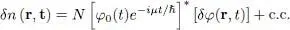
(where c.c. stands for “complex conjugate”). Using (26)and (28), we can finally write:

(36)

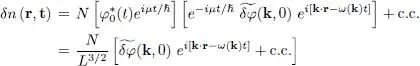
Consequently, the excitation spectrum we have calculated corresponds to density waves propagating in the system with a phase velocity w ( k)/ k .

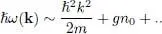
In the absence of interactions, ( g = k 0= 0), this spectrum becomes:

(37)

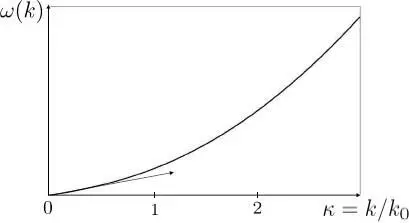
Figure 1: Bogolubov spectrum: variations of the function ω ( k) given by equation (32) as a function of the dimensionless variable κ = k / k 0. When κ ≪ 1, we get a linear spectrum (the arrow in the figure shows the tangent to the curve at the origin), whose slope is equal to the sound velocity c; when κ ≫ 1, the spectrum becomes quadratic, as for a free particle .

which simply yields the usual quadratic relation for a free particle. Physically, this means that the boson system can be excited by transferring a particle from the individual ground state, with wave function φ 0( r) and zero kinetic energy, to any state φk ( r) having an energy ħ 2 k 2/2 m .

In the presence of interactions, it is no longer possible to limit the excitation to a single particle, which immediately transmits it to the others. The system’s excitations become what we call “elementary excitations”, involving a collective motion of all the particles, and hence oscillations in the density of the boson system. If k ≪ k 0, we see from (34)that:

(38)

where c is defined as:

(39)

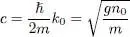
For small values of k , the interactions have the effect of replacing the quadratic spectrum (37)by a linear spectrum. The phase velocity of all the excitations in this k value domain is a constant c . It is called the “sound velocity “ in the interacting boson system, by analogy with a classical fluid where the sound wave dispersion relation is linear, as predicted by the Helmholtz equation. We shall see in § 3 that the quantity c plays a fundamental role in the computations related to superfluidity, especially for the critical velocity determination. If, on the other hand, k ≫ k 0, the spectrum becomes:

(40)

(the following corrections being in , etc.). We find again, within a small correction, the free particle spectrum: exciting the system with enough energy allows exciting individual particles almost as if they were independent. Figure 1shows the complete variation of the spectrum (32), with the transition from the linear region at low energies, to the quadratic region at high energies.

Comment:

As we assumed the interactions to be repulsive in (21), the square roots in (32)and (39)are well defined. If the coupling constant g becomes negative, the sound velocity c will become imaginary, and, as seen from (32), so will the frequencies ω ( k ) (at least for small values of k ). This will lead, for the evolution equation (29), to solutions that are exponentially increasing or decreasing in time, instead of oscillating. An exponentially increasing solution corresponds to an instability of the system. As already encountered in § 4-c of Complement C XV, we see that a boson system becomes unstable in the presence of attractive interactions, however small they might be. In § 4-b of Complement H XV, we shall see that this instability persists even for non-zero temperature. In a general way, an attractive condensate occupying a large region in space tends to collapse onto itself, concentrating into an ever smaller region. However, when it is confined in a finite region (as is the case for experiments where cold atoms are placed in a magneto-optical trap), any change in the wave function that brings the system closer to the instability also increases the gas energy; this results in an energy barrier, which allows the system of condensed attractive bosons to remain in a metastable state.

Let us return to the study of the time evolution of the Gross-Pitaevskii wave function and of the density variations n ( r, t ), without assuming as in § 1-c that the boson system stays very close to uniform equilibrium. We will show that the Gross-Pitaevskii equation can take a form similar to the hydrodynamic equation describing a fluid’s evolution. In this discussion, it is useful to normalize the Gross-Pitaevskii wave function to the particle number, as in equation (17). Equation (16)can then be written as:

(41)

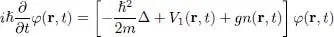
where the local particle density n ( r, t ) is given by:

(42)

Since:

(43)

the time variation of the density may be obtained by first multiplying (41)by φ *( r, t ), then its complex conjugate by φ ( r, t ), and then adding the two results; the potential terms in V 1( r, t ) and g n ( r, t ) cancel out, and we get:

(44)