Claude Cohen-Tannoudji - Quantum Mechanics, Volume 3

We assume that the ket describing the physical system of N bosons can be written using relation (7)of Complement C XV:

(1)

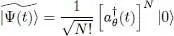
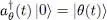
but we now suppose that the individual ket | θ 〉 is a function of time | θ ( t )〉. The creation operator in the corresponding individual state is then time-dependent:

(2)

We will let the ket | θ ( t )〉 vary arbitrarily, as long as it remains normalized at all times:

(3)

We are looking for the time variations of | θ ( t )〉 that will yield for variations as close as possible to those predicted by the exact N -particle Schrodinger equation. As the one-particle potential V 1may also be time-dependent, it will be written as V 1( t ).

Let us introduce the functional of |Ψ( t )〉:

(4)

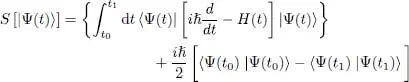
It can be shown that this functional is stationary when |Ψ( t )〉 is solution of the exact Schrodinger equation (an explicit demonstration of this property is given in § 2 of Complement F XV. If |Ψ( t )〉 belongs to a variational family, imposing the stationarity of this functional allows selecting, among all the family kets, the one closest to the exact solution of the Schrodinger equation. We shall therefore try and make this functional stationary, choosing as the variational family the set of kets written as in (1)where the individual ket | θ ( t )〉 is time-dependent.

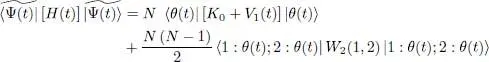
As condition (3)means that the norm of remains constant, the second bracket in expression (4)must be zero. We now have to evaluate the average value of the Hamiltonian H ( t ) that, actually, has been already computed in (34)of Complement C XV:

(5)

The only term left to be computed in (4)contains the time derivative.

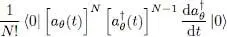
This term includes the diagonal matrix element:

(6)

For an infinitesimal time dt , the operator is proportional to the difference 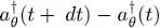, hence to the difference between two creation operators associated with two slightly different orthonormal bases. Now, for bosons, all the creation operators commute with each other, regardless of their associated basis. Therefore, in each term of the summation over k , we can move the derivative of the operator to the far right, and obtain the same result, whatever the value of k . The summation is therefore equal to N times the expression:

(7)

Now, we know that:

(8)

Using in (6)the bra associated with that expression, multiplied by N , we get:

(9)

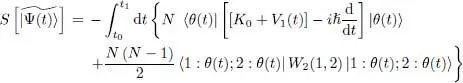
Regrouping all these results, we finally obtain:

(10)

We now make an infinitesimal variation of | θ ( t )〉:

(11)

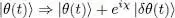
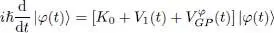
in order to find the kets | θ ( t )〉 for which the previous expression will be stationary. As in the search for a stationary state in Complement C XV, we get variations coming from the infinitesimal ket eiχ | δθ ( t )〉 and others from the infinitesimal bra e –iχ〈 δθ ( t )|; as χ is chosen arbitrarily, the same argument as before leads us to conclude that each of these variations must be zero. Writing only the variation associated with the infinitesimal bra, we see that the stationarity condition requires | θ ( t )〉 to be a solution of the following equation, written for | φ ( t )〉:

(12)

The mean field operator is defined as in relations (45)and (46)of Complement C XVby a partial trace:

(13)

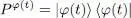
where P φ(t)is the projector onto the ket | φ ( t )〉:

(14)

As we take the trace over particle 2 whose state is time-dependent, the mean field is also time-dependent. Relation (12)is the general form of the time-dependent Gross-Pitaevskii equation.

Let us return, as in § 2 of Complement C XV, to the simple case of spinless bosons, interacting through a contact potential: