Claude Cohen-Tannoudji - Quantum Mechanics, Volume 3

- k = l = m = n = a or b yields the contribution:(65)

- k = m = a and l = n = b, or k = m = b and l = n = a; these two possibilities yield the same contribution (since the W2 operator is symmetric), and the 1/2 factor disappears, leading to the direct term:(66)

- Finally k = n = a and l = m = b, or k = n = b and l = m = a, yield two contributions whose sum introduces the exchange term (here again without the factor 1/2):

(67)

The direct and exchange terms have been schematized in Figure 3 in Chapter XV(replacing | u i〉 by | θ a〉, and | uj 〉 by | θ b〉), with the direct term on the left, and the exchange term on the right.

The variational energy can thus be written as:

(68)

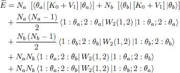
As above, the interaction between particles in the same state | θ a〉 contributes a term proportional to Na ( Na — 1)/2, the number of pairs of particles in that state; the same is true for the interaction term between particles in the same state | θ b〉. The direct term associated with the interaction between two particles in distinct states is proportional to NaNb , the number of such pairs. But to this direct term we must add an exchange term, also proportional to NaNb , corresponding to an additional interaction. This increased interaction is due to the bunching effect of two bosons in different quantum states, that will be discussed in more detail in § 3-b of Complement A XVI. As they are indistinguishable, two bosons occupying individual orthogonal states show correlations in their positions; this increases the probability of finding them at the same point in space. This increase does not occur when the two bosons occupy the same individual quantum state.

We now assume the diagonal matrix elements of [ K 0+ V 1] between the two states | θ a〉 and | θ b〉 to be practically the same. For example, if these two states are the lowest energy levels of spinless particles in a cubic box of edge L , the corresponding energy difference is proportional to 1/ L 2- hence very small in the limit of large L . We also assume all the matrix elements of W 2(1,2) to be equal, which is the case if the (microscopic) range of the particle interaction potential is very small compared to the distances over which the wave functions of the two states vary. We can therefore replace in all the matrix elements the kets | θ a〉 and | θ b〉 by the same ket | θ 〉. Since Na + Nb = N , we obtain:

(69)

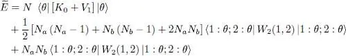
However:

(70)

so that:

(71)

with:

(72)

We find again result (34), but with an additional term , the exchange term. Two cases are then possible, depending on whether the particle interactions are attractive or repulsive. In the first case, the fragmentation of the condensate lowers the energy and leads to a more stable state. Consequently, when the particle interactions are attractive, a condensate where only one individual state is occupied tends to split into two condensates, which might each split again, and so on. This means that the initial single condensate is unstable (we will come back and discuss this instability in § 2-b of Complement F XVfor the more general case of thermal equilibrium at non-zero temperature). On the contrary, for repulsive interactions the fragmentation increases the energy and leads to a less stable state: repulsive interactions therefore tend to stabilize the condensate in a single individual quantum state 5 . This result will be interpreted in § 3-b of Complement A XVIin terms of changes of the particle position correlation function (bunching effect of bosons). As for the ideal gas, an intermediate case between the two previous ones, it is a marginal borderline case: adding any infinitesimal attractive interaction, no matter how small, destabilizes any condensate.

1 1 This means that the stationary condition may be found by varying indifferently the real or imaginary part of θ(r).

2 2 Strictly speaking, in what is generally called the Gross-Pitaevskii equation, the coupling constant g is replaced by 4πħ2a0/m, where a0 is the “scattering length”; this length is defined when studying the collision phase shift δl (k) (Chapter VIII, § C), as the limit of δ0 ~ — ka0 when k → 0. This scattering length is a function of the interaction potential W2(r, r′), but generally not merely proportional to it, as opposed to the matrix elements of W2(r, r′). It is then necessary to make a specific demonstration for this form of the Gross-Pitaevskii equation, using for example the “pseudo-potential” method.

3 3 We use the simpler notation W2(1, 2) for W2(R1, R2).

4 4 A more precise derivation can be given by verifying that is a solution of the one-dimensional equation (56).

5 5 We are discussing here the simple case of spinless bosons, contained in a box. When the bosons have several internal quantum states, and in other geometries, more complex situations may arise where the ground state is fragmented [4].

1 1 Time evolution 1-a Functional variation 1-b Variational computation: the time-dependent Gross-Pitaevskii equation 1-c Phonons and Bogolubov spectrum

2 2 Hydrodynamic analogy 2-a Probability current 2-b Velocity evolution

3 3 Metastable currents, superfluidity 3-a Toroidal geometry, quantization of the circulation, vortex 3-b Repulsive potential barrier between states of different l 3-c Critical velocity, metastable flow 3-d Generalization; topological aspects

In this complement, we return to the calculations of Complement C XV, concerning a system of bosons all in the same individual state. We now consider the more general case where that state is time-dependent. Using a variational method similar to the one we used in Complement C XV, we shall study the time variations of the N -particle state vector. This amounts to using a time-dependent mean field approximation. We shall establish in § 1 a time-dependent version of the Gross-Pitaevskii equation, and explore some of its predictions such as the small oscillations associated with Bogolubov phonons. In § 2, we shall study local conservation laws derived from this equation for which we will give a hydrodynamic analogy, introducing a characteristic relaxation length. Finally, we will show in § 3 how the Gross-Pitaevskii equation predicts the existence of metastable flows and superfluidity.