Claude Cohen-Tannoudji - Quantum Mechanics, Volume 3

(54)

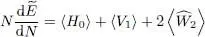
Taking relation (51)into account, this leads to:

(55)

We know ( Appendix VI, § 2-b) that in the grand canonical ensemble, and at zero temperature, the derivative of the energy with respect to the particle number (for a fixed volume) is equal to the chemical potential. The quantity μ introduced mathematically as a Lagrange multiplier, can therefore be simply interpreted as this chemical potential.

The “healing length” is an important concept that characterizes the way a solution of the time-independent Gross-Pitaevskii equation reacts to a spatial constraint (for example, the solution can be forced to be zero along a wall, or along the line of a vortex core). We now calculate an approximate order of magnitude for this length.

Assuming the potential V 1( r) to be zero in the region of interest, we divide equation (28)by φ ( r) and get:

(56)

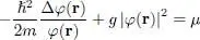
Consequently, the left-hand side of this equation must be independent of r. Let us assume φ ( r) is constant in an entire region of space where the density is n 0, independent of r:

(57)

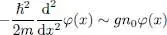
but constrained by the boundary conditions to be zero along its border. For the sake of simplicity, we shall treat the problem in one dimension, and assume φ ( r) only depends on the first coordinate x of r; the wave function must then be zero along a plane (supposed to be at x = 0). We are looking for an order of magnitude of the distance ξ over which the wave function goes from a practically constant value to zero, i.e. for the spatial range of the wave function transition regime. In the region where φ ( r) is constant, relation (56)yields:

(58)

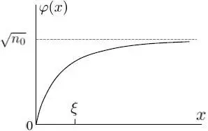
Figure 1: Variation as a function of the position x of the wave function φ ( x ) in the vicinity of a wall (at x = 0) where it is forced to be zero. This variation occurs over a distance of the order of the healing length ξ defined in (61); the stronger the particle interactions, the shorter that length. As x increases, the wave function tends towards a constant plateau, of coordinate , represented as a dashed line .

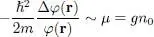
On the other hand, in the whole region where φ ( r) has significantly decreased, and in particular close to the origin, we have:

(59)

In one dimension 4 , we then get the differential equation:

(60)

whose solutions are sums of exponential functions e ±ix/ξ, with:

(61)

The solution that is zero for x = 0 is the difference between these two exponentials; it is proportional to sin( x / ξ ), a function that starts from zero and increases over a characteristic length ξ . Figure 1shows the wave function variation in the vicinity of the wall where it is forced to be zero.

The stronger the interactions, the shorter this “healing length” ξ ; it varies as the inverse of the square root of the product of the coupling constant g and the density n 0. From a physical point of view, the healing length results from a compromise between the repulsive interaction forces, which try to keep the wave function as constant as possible in space, and the kinetic energy, which tends to minimize its spatial derivative (while the wave function is forced to be zero at x = 0); ξ is equal (except for a 2π coefficient) to the de Broglie wavelength of a free particle having a kinetic energy comparable to the repulsion energy gn 0in the boson system.

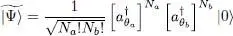
We now show that repulsive interactions do stabilize a boson “condensate” where all the particles occupy the same individual state, as opposed to a “fragmented” state where some particles occupy a different state, which can be very close in energy. Instead of using a trial ket (7), where all the particles form a perfect Bose-Einstein condensate in a single quantum state | θ 〉, we can “fragment” this condensate by distributing the N particles in two distinct individual states. Consequently, we take a trial ket where Na particles are in the state | θ a〉 and Nb = N — Na in the orthogonal state | θ b〉:

(62)

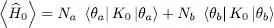
We now compute the change in the average variational energy. In formula (29)giving the average kinetic energy, for the operator to yield a Fock state identical to , we must have either k = l = a , or k = l = b . This leads to:

(63)

The computation of the one-body potential energy is similar and leads to:

(64)

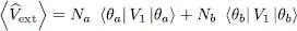
In both cases, the contributions of two populated states are proportional to their respective populations, as expected for energies involving a single particle.

As for the two-body interaction energy, we use again relation (32). It contains the operator , which will reconstruct the Fock state in the following three cases: