Claude Cohen-Tannoudji - Quantum Mechanics, Volume 3

(18)

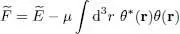
This allows considering the infinitesimal variation δf ( r) to be free of any constraint. The variation of the function is now the sum of 4 variations, coming from the three terms of (16)and from the integral in (18). For example, the variation of yields:

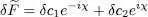
(19)

which is the sum of a term proportional to e –iχand another proportional to e iχ. This is true for all 4 variations and the total variation can be expressed as the sum of two terms:

(20)

the first being the δf *( r) contribution and the second, that of δf ( r). Now if is stationary, must be zero whatever the choice of χ, which is real. Choosing for example χ = 0 imposes δc 1+ δc 2= 0, and the choice χ = π/2 leads (after multiplication by i ) to δc 1— δc 2= 0. Adding and subtracting the two relations shows that both coefficients δc 1and δc 2must be zero. In other words, we can impose to be zero as just θ *( r) varies but not θ ( r) - or the opposite 1 .

We choose to impose the variation to be zero as only θ *( r) varies and for χ = 0. We must first add contributions coming from (13)and (14), then from (15). For this last contribution, we must add two terms, one coming from the variations due to θ *( r′), and the other from the variation due to θ *( r′). These two terms only differ by the notation in the integral variable and are thus equal: we just keep one and double it. We finally add the term due to the variation of the integral in (18), and we get:

(21)

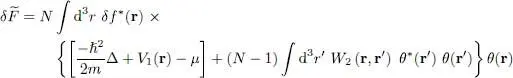
This variation must be zero for any value of δf *( r); this requires the function that multiplies δf *( r) in the integral to be zero, and consequently that θ ( r) be the solution of the following equation, written for φ( r):

(22)

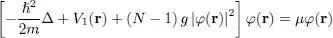
This is the time-independent Gross-Pitaevskii equation. It is similar to an eigenvalue Schrodinger equation, but with a potential term:

(23)

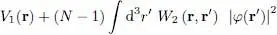
which actually contains the wave function φ in the integral over d 3 r ′; it is therefore a nonlinear equation. The physical meaning of the potential term in W 2is simply that, in the mean field approximation, each particle moves in the mean potential created by all the others, each of them being described by the same wave function φ( r′); the factor ( N — 1) corresponds to the fact that each particle interacts with ( N — 1) other particles. The Gross-Pitaevskii equation is often used to describe the properties of a boson system in its ground state (Bose-Einstein condensate).

The Gross-Pitaevskii equation is often written in conjunction with an approximation where the particle interaction potential has a microscopic range, very small compared to the distances over which the wave function φ ( r) varies. We can then substitute:

(24)

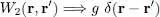
where the constant g is called the “coupling constant”; such a potential is sometimes known as a “contact potential” or, in other contexts, a “Fermi potential”. We then get:

(25)

Whether in this form 2 or in its more general form (22), the equation includes a cubic term in φ ( r). It may render the problem difficult to solve mathematically, but it also is the source of many interesting physical phenomena. This equation explains, for example, the existence of quantum vortices in superfluid liquid helium.

Rather than normalizing the wave function φ ( r) to 1 in the entire space, one sometimes chooses a normalization taking into account the particle number by setting:

(26)

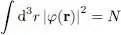
This amounts to multiplying by the wave function we have used until now. At each point rof space, the particle (numerical) density n ( r) is then given by:

(27)

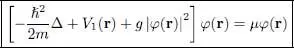
With this normalization, the factor ( N — 1) in (25)is replaced by ( N — 1)/ N , which can generally be taken equal to 1 for large N . The Gross-Pitaevskii equation then becomes:

(28)