Claude Cohen-Tannoudji - Quantum Mechanics, Volume 3

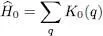
The first term is simply the sum of the individual kinetic energy operators associated with each of the particles q :

(2)

where:

(3)

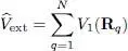
( P qis the momentum of particle q ). Similarly, is the sum of the external potential operators V 1( R q), each depending on the position operator R qof particle q :

(4)

Finally, is the sum of the interaction energy associated with all the pairs of particles:

(5)

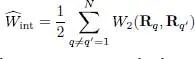
(this summation can also be written as a sum over q < q ′, while removing the prefactor 1/2).

Let us choose an arbitrary normalized quantum state | θ 〉:

(6)

and call the associated creation operator. The N -particle variational kets we consider are defined by the family of all the kets that can be written as:

(7)

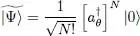
where | θ 〉 can vary, only constrained by (6). Consider a basis {| θ k〉} of the individual state space whose first vector is | θ 1〉 = | θ 〉. Relation (A-17) of Chapter XVshows that this ket is simply a Fock state whose only non-zero occupation number is the first one:

(8)

An assembly of bosons that occupy the same individual state is called a “Bose-Einstein condensate”.

Relation (8)shows that the kets are normalized to 1. We are going to vary | θ 〉, and therefore , so as to minimize the average energy:

(9)

We start with a simple case where the bosons have no spin. We can then use the wave function formalism and keep the computations fairly simple.

Assuming one single individual state to be populated, the wave function Ψ( r 1, r 2,…, r N) is simply the product of N functions θ ( r):

(10)

with:

(11)

This wave function is obviously symmetric with respect to the exchange of all particles and can be used for a system of identical bosons.

In the position representation, each operator K 0( q ) defined by (3)corresponds to (—ħ 2/2 m ) Δ rq, where Δ rqis the Laplacian with respect to the position r q; consequently, we have:

(12)

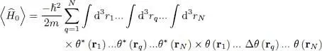
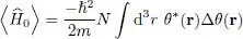
In this expression, all the integral variables others than r qsimply introduce the square of the norm of the function θ ( r), which is equal to 1. We are just left with one integral over r q, in which r qplays the role of a dummy variable, and thus yields a result independent of q . Consequently, all the q values give the same contribution, and we can write:

(13)

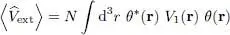
As for the one-body potential energy, a similar calculation yields:

(14)

Finally, the interaction energy calculation follows the same steps, but we must keep two integral variables instead of one. The final result is proportional to the number N ( N — 1)/2 of pairs of integral variables:

(15)

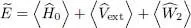
The variational average energy is the sum of these three terms:

(16)

We now optimize the energy we just computed, so as to determine the wave functions θ ( r) corresponding to its minimum value.

Let us vary the function θ ( r) by a quantity:

(17)

where δf ( r) is an infinitesimal function and χ an arbitrary number. A priori, δ f ( r) must be chosen to take into account the normalization constraint (6), which forces the integral of the θ ( r) modulus squared to remain constant. We can, however, use the Lagrange multiplier method (Appendix V) to impose this constraint. We therefore introduce the multiplier μ (we shall see in § 4-a that this factor can be interpreted as the chemical potential) and minimize the function: