Claude Cohen-Tannoudji - Quantum Mechanics, Volume 3

As μ gets closer to zero, the population N 0of the ground state becomes:

(63)

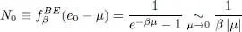
This population diverges in the limit μ = 0 and, when | μ | gets small enough, it can become arbitrarily large. It can, for example, become proportional 5 to the volume , in which case it adds a finite contribution to the particle numerical density (particle number per unit volume) as .

This particularity is limited to the ground state, which, in this case, plays a very different role than the other levels. Let us show, for example, that the first excited state population does not yield a similar effect. Assuming the system to be contained in a cubic box 6 of edge length L , the population of the first excited energy level e 1~ π 2 ħ 2/(2 mL 2) can be written as:

(64)

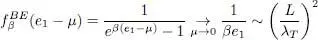
(we assume the box to be large enough so that L ≫ λ T, which means βe 1≪ 1); this population can therefore be proportional only to the square of L , i.e. to the volume to the power 2/3. It shows that this first excited level cannot make a contribution to the particle density in the limit L → ∞; the same is true for all the other excited levels whose contributions are even smaller. The only arbitrary contribution to the density comes from the ground state.

This arbitrarily large value as μ → 0 obviously does not appear in relation (59), which predicts that the density 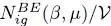is always less than a finite value as shown by (62). This is not surprising: as the population varies radically from the first energy level to the next, we can no longer compute the average particle number by replacing in (55)the discrete summation by an integral and a more precise calculation is necessary. Actually, only the ground state population must be treated separately, and the summation over all the excited states (of which none contributes to the density divergence) can still be replaced by an integral as before. Consequently, to get the total population of the physical system we simply add the integral on the right-hand side of (57)to the contribution N 0of the ground level:

(65)

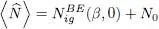
where N 0is defined in (63).

As μ → 0, the total population of all the excited levels (others than the ground level) remains practically constant and equal to its upper limit (62); only the ground state has a continuously increasing population N 0, which becomes comparable to the total population of all the excited states when the right-hand sides of (63)and (62)are of the same order of magnitude:

(66)

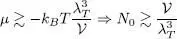
( μ being of course always negative). When this condition is satisfied, a significant fraction of the particles accumulates in the individual ground level, which is said to have a “macroscopic population” (proportional to the volume). We can even encounter situations where the majority of the particles all occupy the same quantum state. This phenomenon is called “Bose-Einstein condensation” (it was predicted by Einstein in 1935, following Bose’s studies of quantum statistics applicable to photons). It occurs when the total density ntot reaches the maximum predicted by formula (62), that is:

(67)

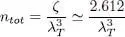
This condition means that the average distance between particles is of the order of the thermal wavelength λ T.

Initially, Bose-Einstein condensation was considered to be a mathematical curiosity rather than an important physical phenomenon. Later on, people realized that it played an important role in superfluid liquid Helium 4, although this was a system with constantly interacting particles, hence far from an ideal gas. For a dilute gas, Bose-Einstein condensation was observed for the first time in 1995, and in a great number of later experiments.

The “equation of state” of a fluid at thermal equilibrium is the relation that links, for a given particle number N , its pressure P , volume V , and temperature T = 1/ kBβ . We have just studied the variations of the total particle number. We shall now examine the pressure of a fermion or boson ideal gas.

The grand canonical potential of a fermion ideal gas is given by (9). Equation (14)indicates that, for a system at thermal equilibrium, this grand potential is equal to the opposite of the product of the volume and the pressure P . We thus have:

(68)

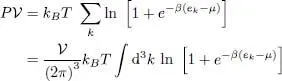
(where the second equality is valid in the limit of large volumes). Simplifying by , we get the pressure of a fermion system contained in a box of macroscopic dimension:

(69)

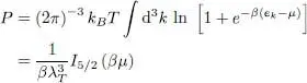
with:

(70)

where x has been defined in (53).

To obtain the equation of state, we must find a relation between the pressure P , the volume , and the temperature T of the physical system, assuming the particle number to be fixed. We have, however, used the grand canonical ensemble (cf. Appendix VI), where the temperature is determined by the parameter β and the volume is fixed, but where the particle number can vary: its average value is a function of a parameter, the chemical potential μ (for fixed values of μ and ). Mathematically, the pressure P appears as a function of , T and μ and not as the function of , T and the particle number we were looking for. We can nevertheless vary μ , and obtain values of the pressure and particle number of the system and consequently explore, point by point, the equation of state in this parametric form. To obtain an explicit form of the equation of state would require the elimination of the chemical potential using both (47)and (69); there is generally no algebraic solution, and people just use the parametric form of the equation of state, which allows computing all the possible state variables. There also exists a “virial expansion” in powers of the fugacity eβμ , which allows the explicit elimination of μ at all the successive orders; its description is beyond the scope of this book.